proj3/
Image Warping and Mosaicing!
Overview
This project explores two fundamental computer vision techniques: image warping and mosaicing (Part A), and feature detection and matching (Part B). In Part A, we implement homography computation from point correspondences, perform inverse warping with nearest-neighbor and bilinear interpolation, and blend multiple images into seamless mosaics. In Part B, we develop automatic feature detection and matching algorithms to create mosaics without manual point selection.
Part A: Image Warping and Mosaicing
A.1: Shoot and Digitize Pictures
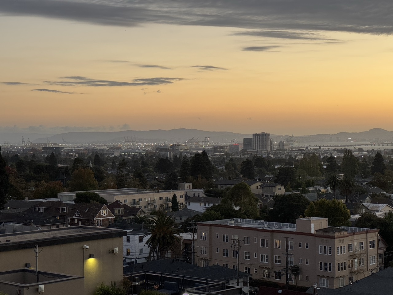
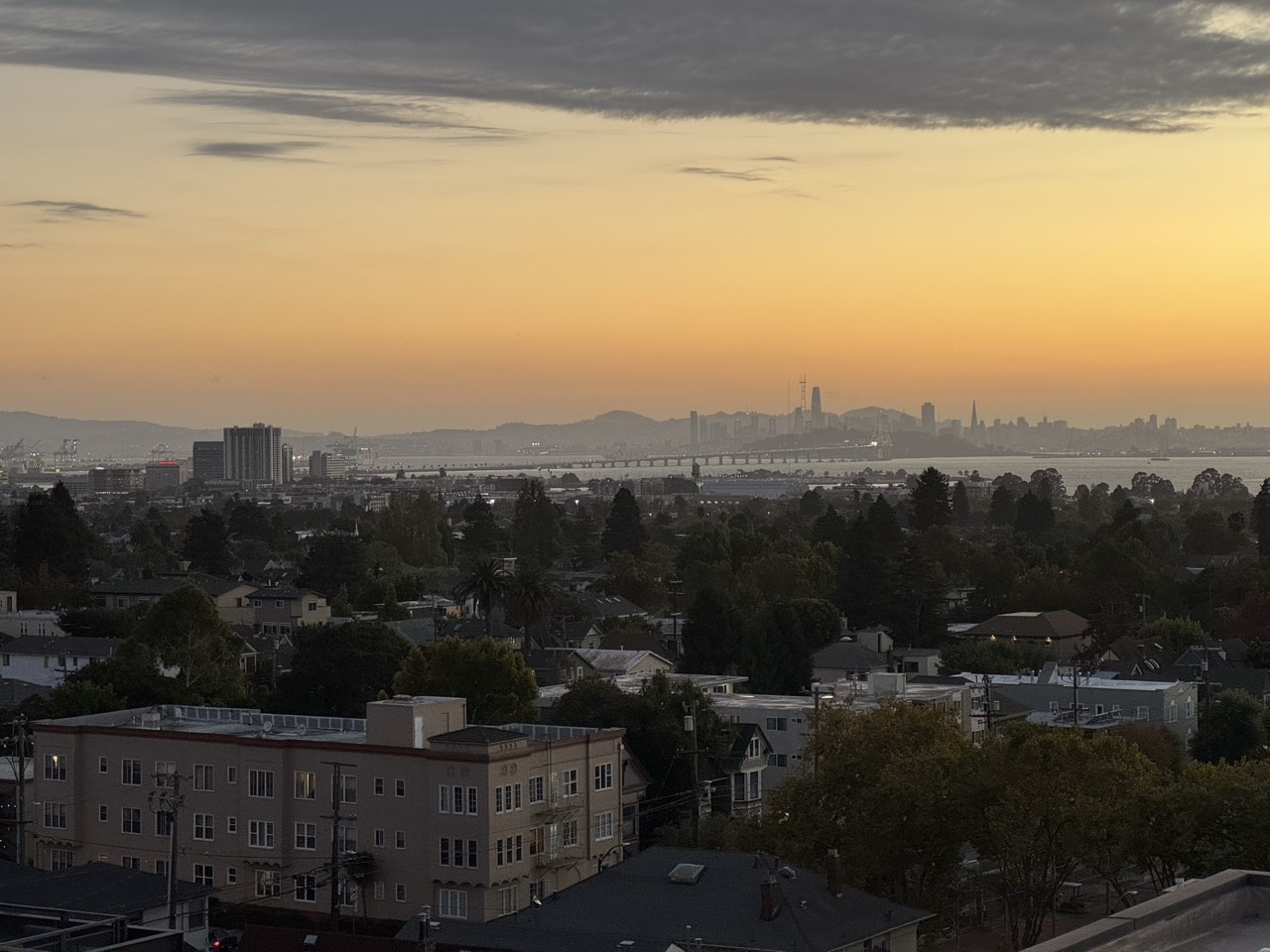
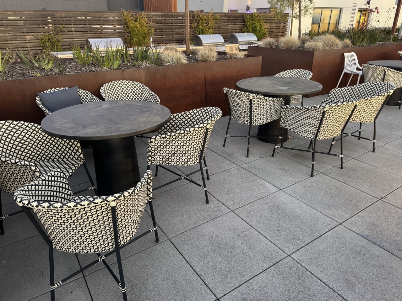
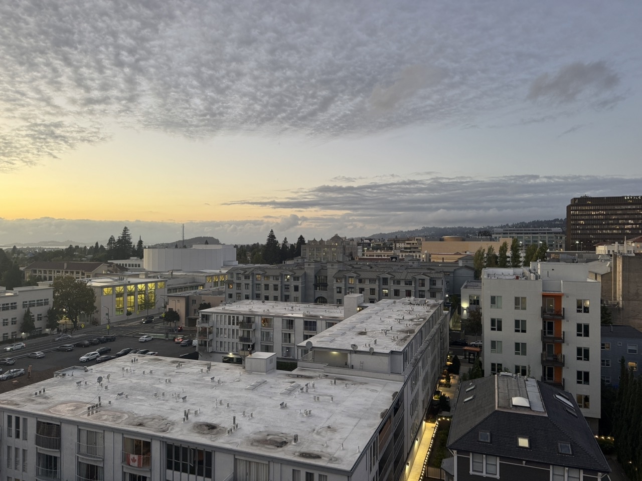
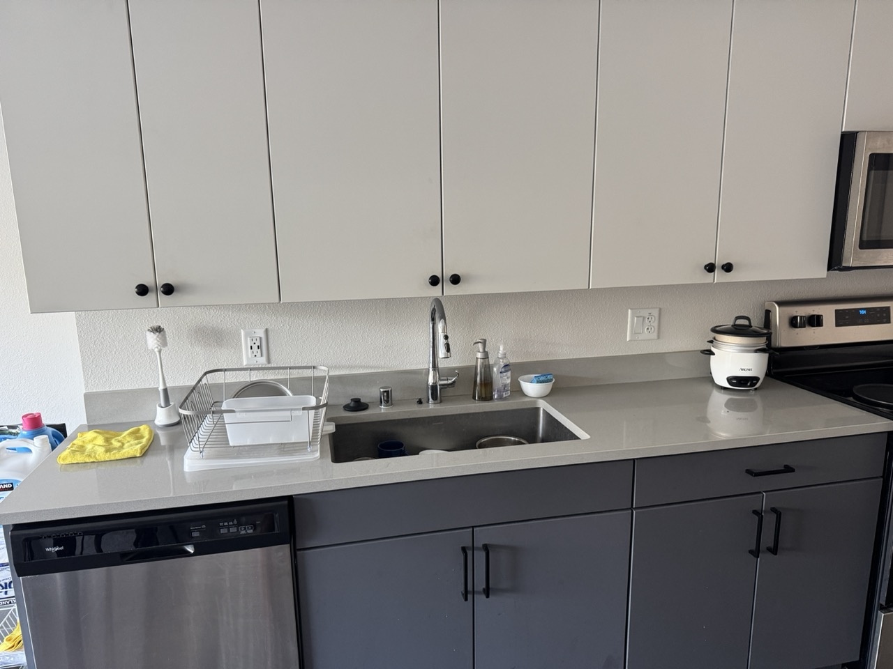
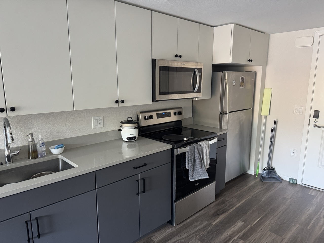
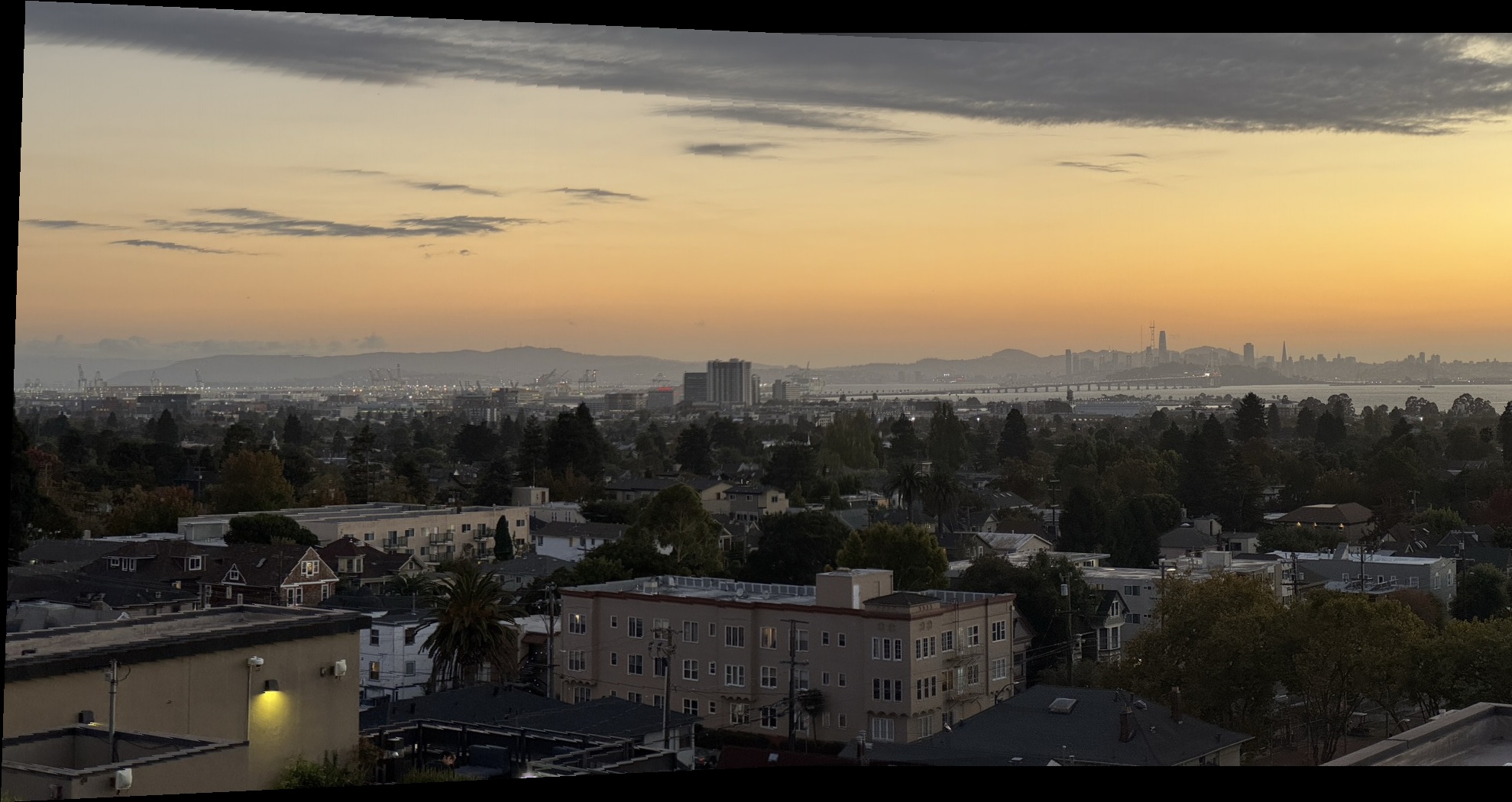
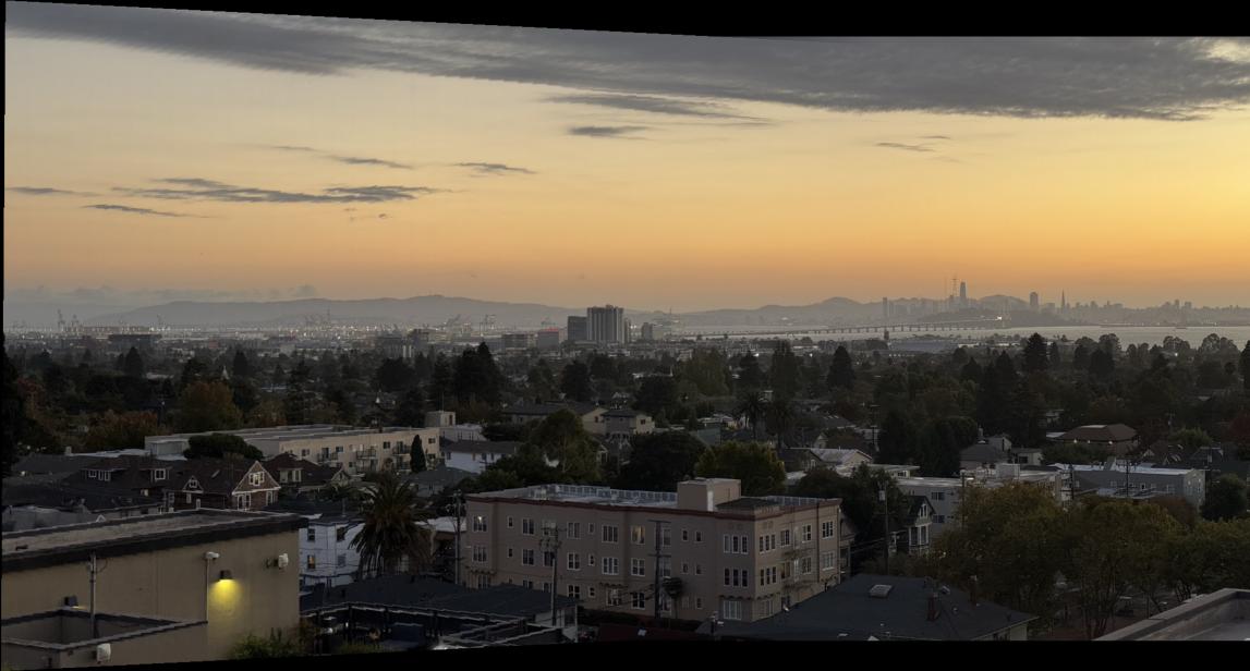
I collected four pairs of images with projective transforms between them, each with 40-70% overlap. Below are the source and reference image pairs used for warping and mosaicing. Each pair was captured with a fixed center of projection while rotating the camera.
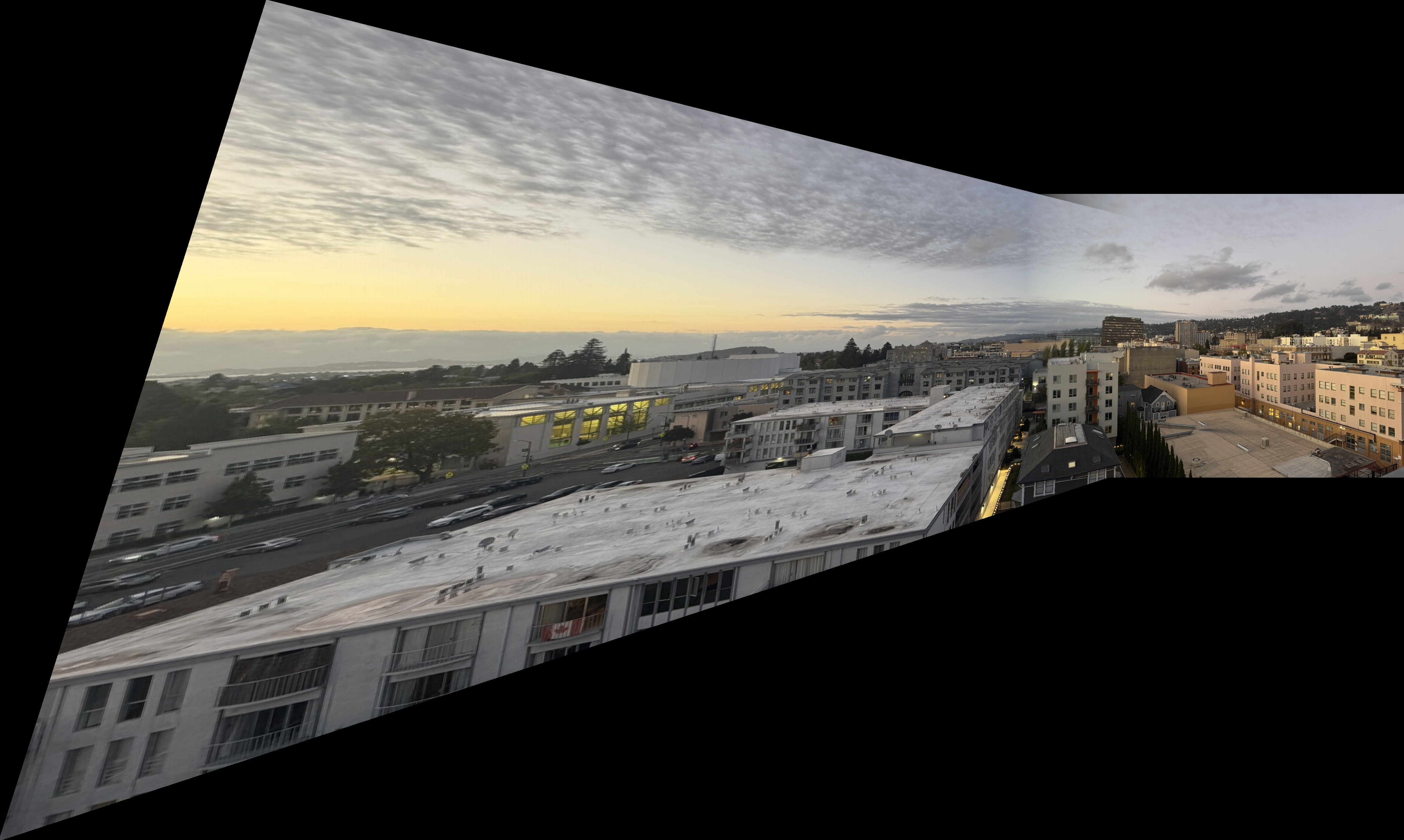
Bay Scene
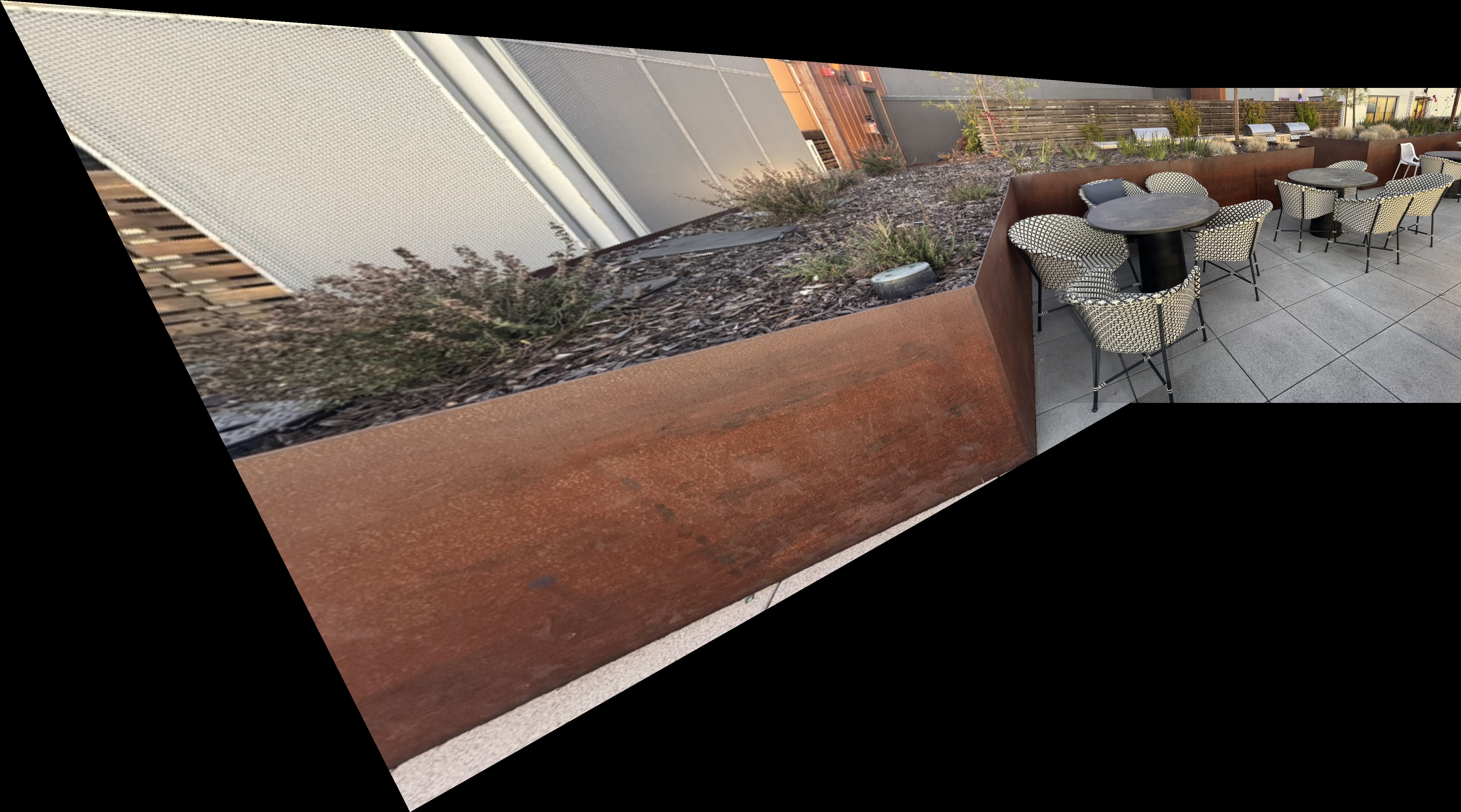
Outdoor Chairs

Downtown Scene
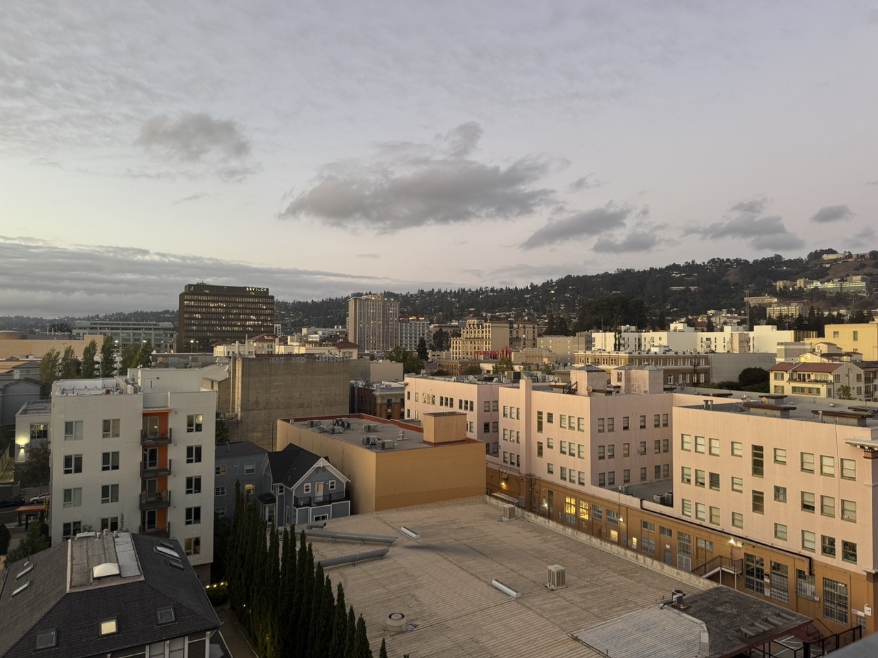
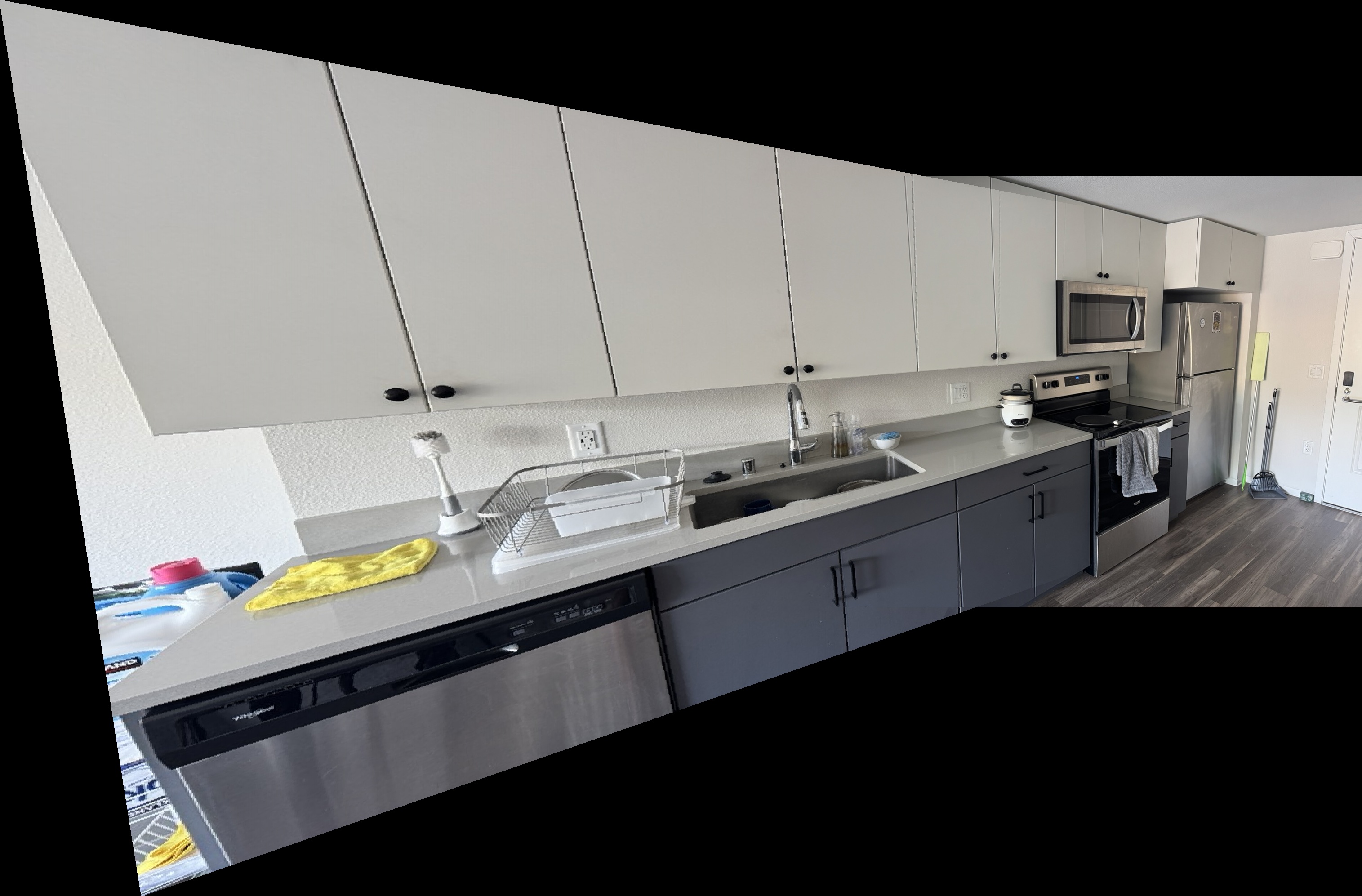
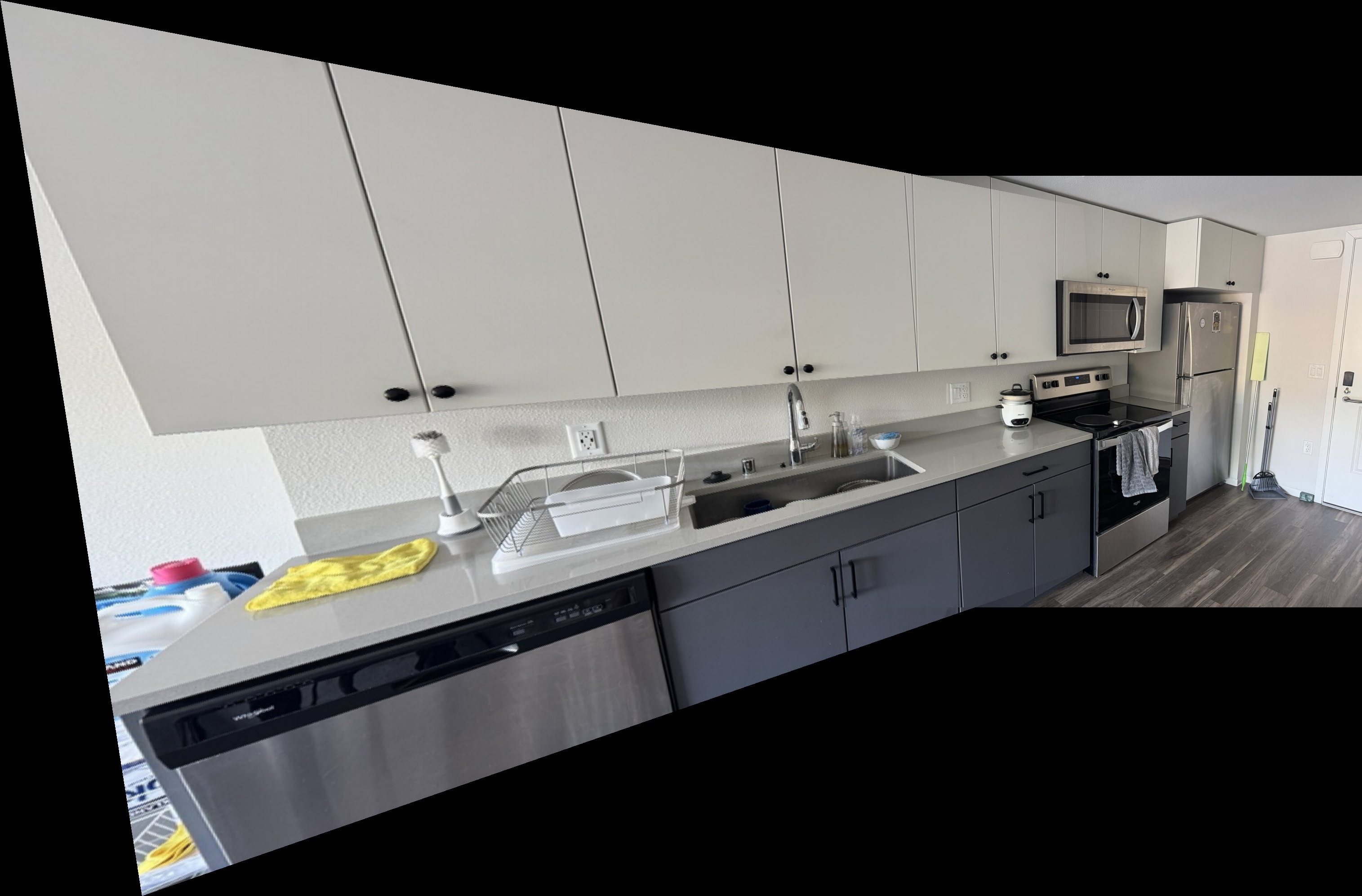
Kitchen Sink
A.2: Recover Homographies
For this section, I implemented the function H = computeH(im1_pts, im2_pts) to recover the
transformation matrix between a source image and its corresponding image. The mapping follows the equation:
$p' = Hp$ where $p = [x,\; y,\; 1]^T$ represents a point in the source image and
$p' = [x',\; y',\; 1]^T$ represents the corresponding point in the destination image.
The goal is to estimate $H$, a $3\times 3$ matrix with 8 degrees of freedom (since one element can be fixed to 1).
Building the System of Equations
Each correspondence provides two linear equations derived from:
\begin{align*} x' &= \frac{h_{11}x + h_{12}y + h_{13}}{h_{31}x + h_{32}y + 1} \\[10pt] y' &= \frac{h_{21}x + h_{22}y + h_{23}}{h_{31}x + h_{32}y + 1} \end{align*}
Rearranging these gives a linear system in the form \(A h = b\), where each point correspondence contributes two rows to $A$ and $b$. For clarity, below is the explicit 8-row system that results from four point correspondences (\((x_i,y_i)\) ↦ \((x'_i,y'_i)\), \(i=1\ldots4\)):
$$ A = \begin{bmatrix} x_1 & y_1 & 1 & 0 & 0 & 0 & -x_1 x'_1 & -y_1 x'_1 \\ 0 & 0 & 0 & x_1 & y_1 & 1 & -x_1 y'_1 & -y_1 y'_1 \\ x_2 & y_2 & 1 & 0 & 0 & 0 & -x_2 x'_2 & -y_2 x'_2 \\ 0 & 0 & 0 & x_2 & y_2 & 1 & -x_2 y'_2 & -y_2 y'_2 \\ x_3 & y_3 & 1 & 0 & 0 & 0 & -x_3 x'_3 & -y_3 x'_3 \\ 0 & 0 & 0 & x_3 & y_3 & 1 & -x_3 y'_3 & -y_3 y'_3 \\ x_4 & y_4 & 1 & 0 & 0 & 0 & -x_4 x'_4 & -y_4 x'_4 \\ 0 & 0 & 0 & x_4 & y_4 & 1 & -x_4 y'_4 & -y_4 y'_4 \end{bmatrix},\qquad h = \begin{bmatrix} h_{11} \\ h_{12} \\ h_{13} \\ h_{21} \\ h_{22} \\ h_{23} \\ h_{31} \\ h_{32} \end{bmatrix},\qquad b = \begin{bmatrix} x'_1 \\ y'_1 \\ x'_2 \\ y'_2 \\ x'_3 \\ y'_3 \\ x'_4 \\ y'_4 \end{bmatrix} $$
$$A\,h = b$$
After stacking all n correspondences, we get an overdetermined system. Since small errors in the point matches can lead to large variations in $H$, I solved this system using a least-squares approach to minimize error:
$$h = (A^{T}A)^{-1}A^{T}b$$
I then appended 1.0 as the final entry of $h$ and reshaped it into a $3×3$ homography matrix $H$. This normalization ensures that $H[2,2] = 1$.
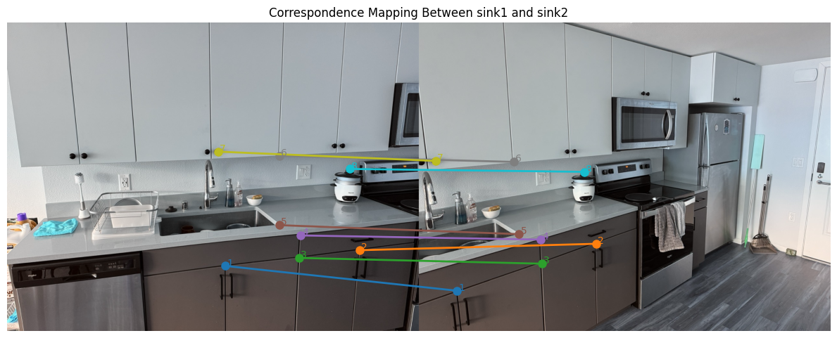
Sink correspondence visualization, assembled system, and recovered H
Below are the source/reference images used for the sink correspondences, the assembled linear system \(A\) built from the eight point matches, and the final recovered homography \(H\).
_
Matrix A (16×8)
$$ A = \begin{bmatrix} 678 & 757 & 1 & 0 & 0 & 0 & -79326 & -88569 \\ 0 & 0 & 0 & 678 & 757 & 1 & -565452 & -631338 \\ 1096 & 708 & 1 & 0 & 0 & 0 & -603896 & -390108 \\ 0 & 0 & 0 & 1096 & 708 & 1 & -754048 & -487104 \\ 907 & 732 & 1 & 0 & 0 & 0 & -346474 & -279624 \\ 0 & 0 & 0 & 907 & 732 & 1 & -680250 & -549000 \\ 911 & 662 & 1 & 0 & 0 & 0 & -344358 & -250236 \\ 0 & 0 & 0 & 911 & 662 & 1 & -614925 & -446850 \\ 846 & 630 & 1 & 0 & 0 & 0 & -263106 & -195930 \\ 0 & 0 & 0 & 846 & 630 & 1 & -556668 & -414540 \\ 846 & 414 & 1 & 0 & 0 & 0 & -248724 & -121716 \\ 0 & 0 & 0 & 846 & 414 & 1 & -366318 & -179262 \\ 655 & 401 & 1 & 0 & 0 & 0 & -34060 & -20852 \\ 0 & 0 & 0 & 655 & 401 & 1 & -281650 & -172430 \\ 1065 & 455 & 1 & 0 & 0 & 0 & -546345 & -233415 \\ 0 & 0 & 0 & 1065 & 455 & 1 & -494160 & -211120 \end{bmatrix} $$
Vector b (16×1)
$$ b = \begin{bmatrix} 117 \\ 834 \\ 551 \\ 688 \\ 382 \\ 750 \\ 378 \\ 675 \\ 311 \\ 658 \\ 294 \\ 433 \\ 52 \\ 430 \\ 513 \\ 464 \end{bmatrix} $$
Recovered Homography (H)
$$ H = \begin{bmatrix} 2.70952308 & 1.82219090 * 10^{-1} & -1.74977712 * 10^{3} \\ 4.44075072 * 10^{-1} & 2.24081933 & -3.90934467 * 10^{2} \\ 1.25176295 * 10^{-3} & 1.02030528 * 10^{-4} & 1.00000000 \end{bmatrix} $$
A.3: Warp the Images
This part consisted of implementing inverse warping with two interpolation methods from scratch:
- Nearest neighbor: Round source coordinates to the nearest pixel.
warpImageNearestNeighbor(im, H)
- Bilinear: Weighted average of four neighboring pixels.
warpImageBilinear(im, H)
Now that we have our homography matrix from the previous part, we can apply it on our images and be warp them. I implemented two warping mechanisms, which have a key distiction when it comes to choosing pixel values, but everything up until then is similar. First, I predicted the bounding box of an input image by piping the four corners of the image through the computed homography matrix. From here, we get the newly projected corners for the source image in the new output image, which we can use to determine the shape of the complete output mosaic. Initially, the mosaic is zero-filled, meaning its a black canvas. To fill the mosaic, we have to using inverse-warping to retrieve the pixel values from the original source image, and this is where the difference in the nearest-neighbor and bilinear mechanisms come in.
Nearest Neighbor Interpolation
Nearest Neighbor interpolation assigns the value of the closest pixel to the computed source location. This is done by taking the inverse of the homography matrix $H$ and applying it to the newly projected image as mentioned above. However, when taking the inverse, the $(x, y)$ pixel values are not guaranteed to be exact integer values. To overcome this, the nearest neighbor approach just takes the closest pixel to the inverse-calculated pixel, and sets the pixel value in the mosaic image to the value of the closest pixel in the source image. One thing to note is the pixel value was only chosen if the mapped back value was in the bounds of the source image.
For example, given a pixel location $(x_m, y_m)$ in the mosaic, we first compute its corresponding location in the source image
using the inverse homography:
$$p_s = H^{-1} \, p_m = H^{-1} \, \begin{bmatrix} x_m \\ y_m \\ 1 \end{bmatrix} =
\begin{bmatrix} x_s' \\ y_s' \\ w \end{bmatrix},$$
Since $(x_s,y_s)$ are generally not integers, the nearest neighbor method locates the pixel position by rounding:
$$x_{NN} = \\{round}(x_s), \\y_{NN} = \\{round}(y_s).$$
Finally, the pixel value at $(x_{NN},y_{NN})$ in the source image is assigned to the mosaic pixel at $(x_m,y_m)$. This rounding-based calculation, while computationally simple, results in a less smooth output compared to interpolation methods that weight nearby pixel values.
Bilinear Interpolation
Bilinear interpolation computes a weighted average of the four nearest pixels based on the distance from the source location. If we do the same procedure as the nearest neighbors where we take the inverse of the homography matrix and apply it on the mosaic pixel coordinate pair $(x_m, y_m),$ we get the corresponding location in the source image: $(x_s, y_s).$ From here, we can apply bilinear interpolation which takes the pixel values of all the 4 closest pixels around $(x_s, y_s),$ and sets the value of $(x_s, y_s)$ to be the weighted average of all 4 pixel values. Bilinear interpolation may require more computation than nearest neighbors, but it results in a smoother image in the end. One thing to note is the pixel value was only chosen if the mapped back value was in the bounds of the source image.
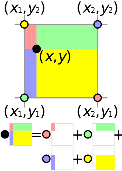
$$ x_1 = \lfloor x_s \rfloor,\quad x_2 = x_1 + 1,\quad y_1 = \lfloor y_s \rfloor,\quad y_2 = y_1 + 1 $$
$$ a = x_s - x_1,\qquad b = y_s - y_1 $$
$$ \begin{aligned} I(x_s, y_s) &= (1 - a)(1 - b)\,I(y_1, x_1) + a(1 - b)\,I(y_1, x_2) \\\\ &\quad + (1 - a)b\,I(y_2, x_1) + a b\,I(y_2, x_2) \end{aligned} $$
Note: I(x, y) represents the image intensity (pixel value) at coordinates (x, y).
Both of these approaches had their strenghts and weaknesses. The nearest neighbors approach was generally faster, less computationally intensive, and less blurry than the bilinear interpolation method. However, bilinear interpolation produced more smooth results due to the weighted blending of surrounding pixel values. On the images below, we can notice the differences in results. For the rectified door, the shadow on the left side of the door is much more linear and smooth in bilinear interpolation. In the nearest neighbors, the shadow outline is more jagged. However, in the table rectified image, the bilinear interpolation is more blurry than the nearest neighbor result.
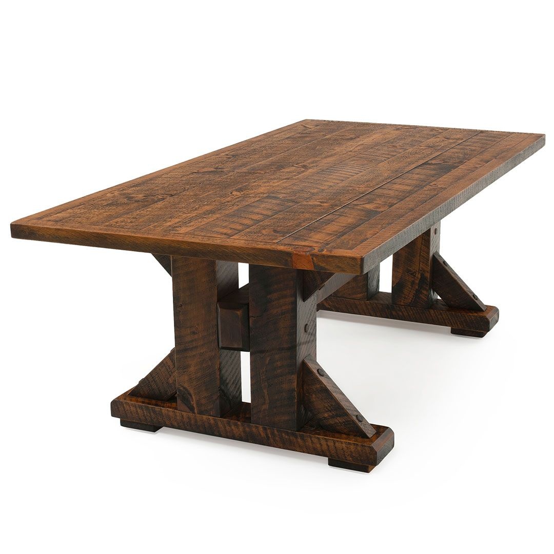
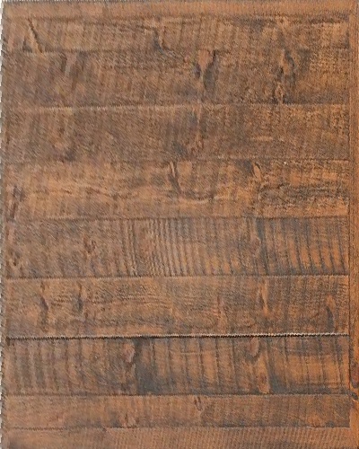
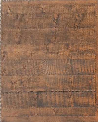
Door Rectification
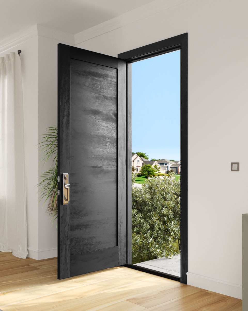
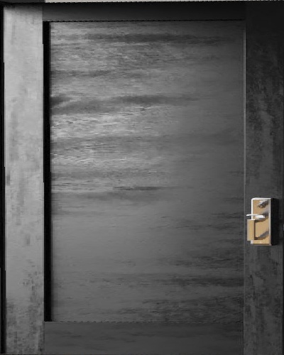
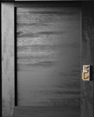
Table Rectification
A.4: Blend the Images into a Mosaic
After warping, now its time to blend the images together, and to do this, I used weighted averaging with alpha masks. The first step to doing this was computing the overall size of the combined mosaic image based on the bounding boxes of the reference and warped images. Each image was also then assigned an alpha mask that takes the value of 1 near the image center and decays linearly towards the edges, creating a smooth alpha mask effect. The blending process then combines both images by taking the weighted sum of their overlapping regions, which is then normalized by the accumulated alpha values.
$$ I_{\text{mosaic}}(x, y) = \frac{\alpha_1(x, y)\,I_1(x, y) + \alpha_2(x, y)\,I_2(x, y)} {\alpha_1(x, y) + \alpha_2(x, y)} $$
Note: \(I_1, I_2\) are the source and warped images, and \(\alpha_1, \alpha_2\) are their corresponding alpha weights that decay toward the edges.
The result is a smooth transition between overlapping regions, resulting in the final mosaic of the two images. Below are the final mosaic results for each dataset, comparing nearest neighbor versus bilinear interpolation mosaics.
Bay Scene Mosaics

Outdoor Chairs Mosaics

Downtown Mosaics

Kitchen Sink Mosaics
Part B: Feature Detection and Matching
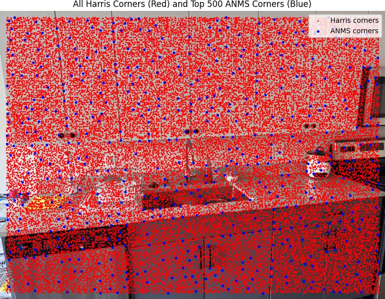
B.1: Harris Corner Detection
The Harris corner detector identifies corners by analyzing local intensity variations. Corners have large intensity changes in multiple directions, unlike edges (one direction) or flat regions (minimal changes).
We build the structure tensor $M$ by accumulating gradient information over a local window:
$$ M = \sum_{(x,y) \in W} \begin{bmatrix} I_x^2 & I_x I_y \\ I_x I_y & I_y^2 \end{bmatrix} $$
The structure tensor can be diagonalized to reveal principal directions of intensity change:
$$ M = R^{-1} \begin{bmatrix} \lambda_1 & 0 \\ 0 & \lambda_2 \end{bmatrix} R $$
where $\lambda_1$ and $\lambda_2$ are eigenvalues representing gradient magnitudes. The Harris corner response is:
$$ R = \frac{\det(M)}{\text{trace}(M)} = \frac{\lambda_1 \lambda_2}{\lambda_1 + \lambda_2} $$
This is maximized when both eigenvalues are large (corners), small when one is large (edges), and very small when both are small (flat regions).
Implementation Results
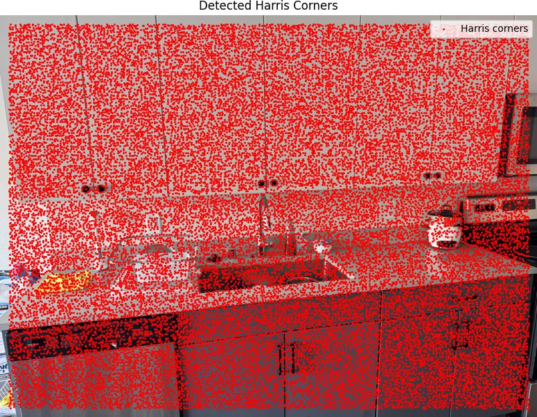
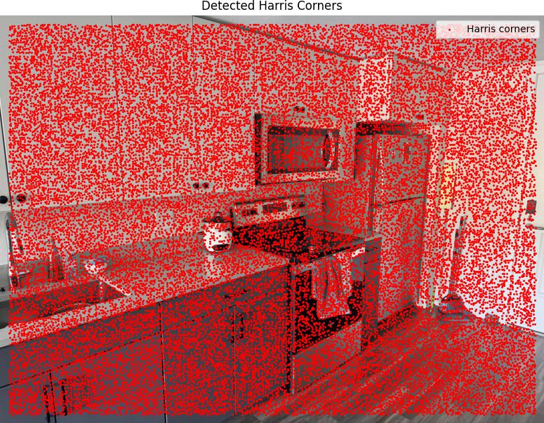
We ran the Harris corner detection algorithm with edge_discard = 20 and min_distance = 1,
which generated 33,265 Harris detections across the images.
Harris Corners Detection Results
Below are the detected Harris corners overlaid on the source images:
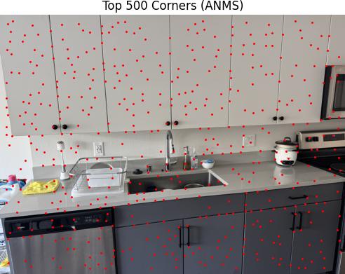
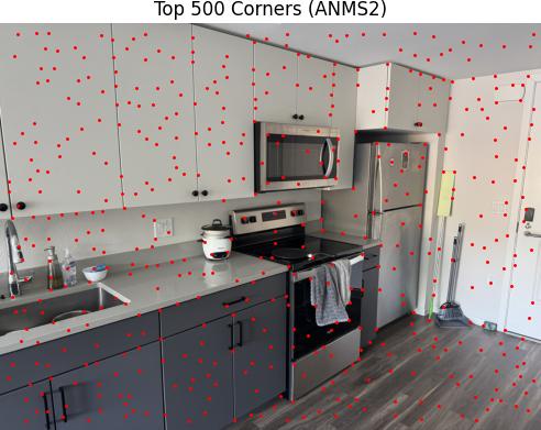
Adaptive Non-Maximal Suppression (ANMS)
ANMS ensures well-distributed corner points by maintaining minimum distances between selected points. Once an interest point appears, it will always remain in the list because if a point is a maximum in radius $r$, it is also a maximum in radius $r' < r$.
In practice, we robustify the non-maximal suppression by requiring that a neighbor has a sufficiently larger strength. The minimum suppression radius $r_i$ is given by:
$$ r_i = \min_j |x_i - x_j|, \quad \text{s.t. } f(x_i) < c_{\text{robust}} f(x_j), \quad x_j \in I $$
where $x_i$ is a 2D interest point image location, and $I$ is the set of all interest points. This reduced the 33,265 Harris detections to 500 well-distributed corners.
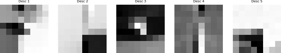
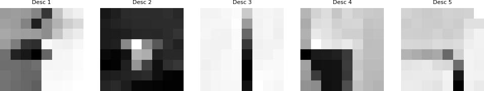
B.2: Feature Descriptor Extraction
In this part I extracted the features of the detected corners by taking a 40×40 window around the corner coordinates. For each corner, I applied Gaussian blur to the 40×40 patch, then sampled every 5th pixel to create the 8×8 descriptor, and finally computed the mean and standard deviation to normalize the descriptor.
Extracted Feature Descriptors
Below are examples of the extracted normalized 8x8 feature descriptors:
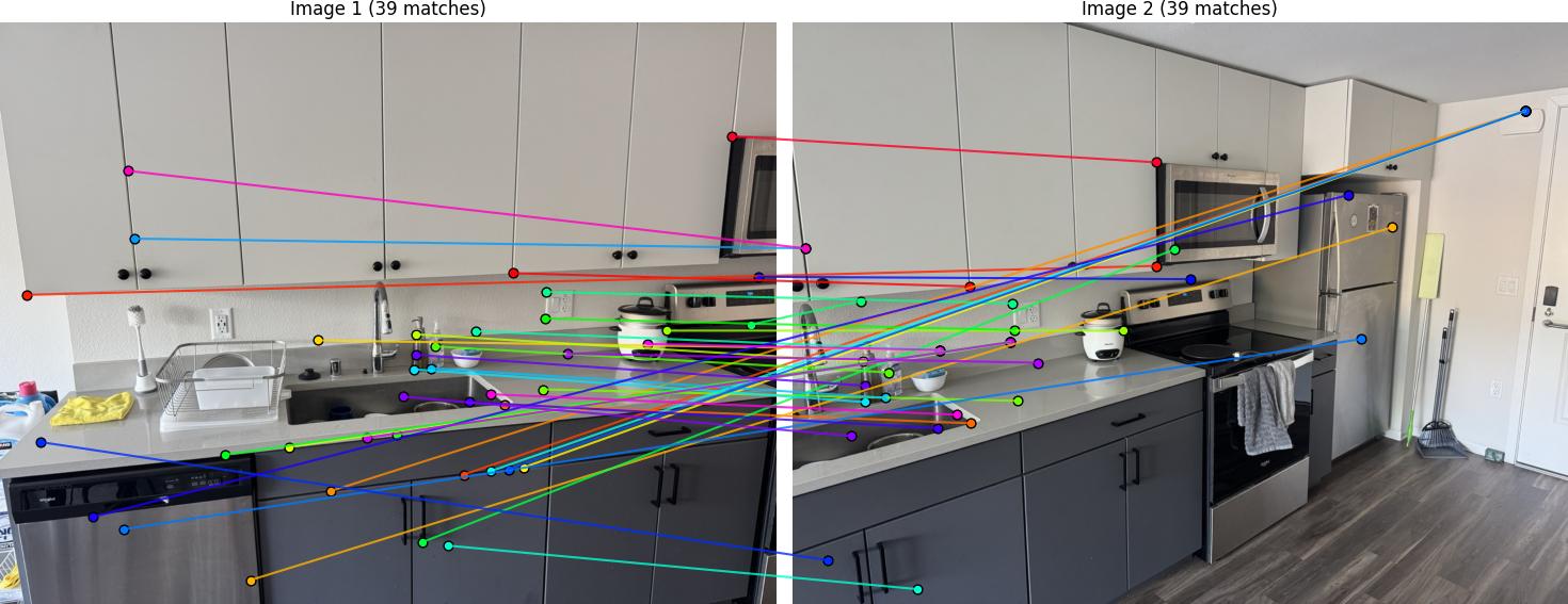
B.3: Feature Matching
I implemented feature matching following Section 5 of the paper. The matching process uses normalized cross-correlation to find similar feature descriptors between image pairs. I used Lowe's ratio test for thresholding, comparing the ratio between the first and second nearest neighbors to filter out ambiguous matches.
For each feature descriptor in image 1, I computed the Euclidean distance to all descriptors in image 2:
$$ d = \|f_2 - f_1\|_2 $$
I found the best and second-best matches, then applied Lowe's ratio test:
$$ \text{ratio} = \frac{d_{\text{best}}}{d_{\text{second}}} $$
If this ratio was less than 0.7, I accepted the match.
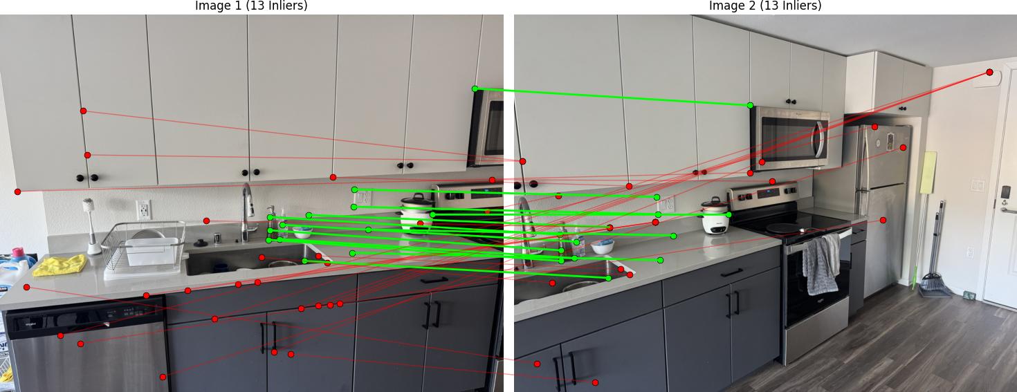
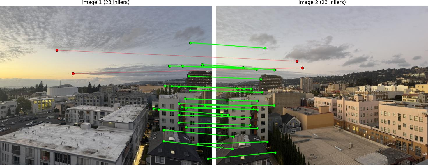
Feature Matching Results
Below are the matched features between image pairs:
B.4: RANSAC for Robust Homography
I implemented 4-point RANSAC to compute robust homography estimates from the matched features. RANSAC (Random Sample Consensus) is essential for handling outliers in feature matches and ensuring reliable homography computation.
RANSAC follows this iterative process to find the best homography:
For each iteration, I get 4 random points from the matched features, then compute the homography from these 4 points. Next, I apply this homography to all points in the first image to project them onto the second image. I then compute the Euclidean distance between the projected points and the actual corresponding points in the second image:
$$ \text{distance} = \|\text{projected} - \text{pts2}\|_2 $$
Points with distance less than $\epsilon = 3.0$ are considered inliers. I count the total number of inliers and compare it to the best inlier count so far. If this iteration has more inliers, I store this as the best homography. After $N = 1000$ iterations, I recompute the final homography using all inlier points from the best iteration.
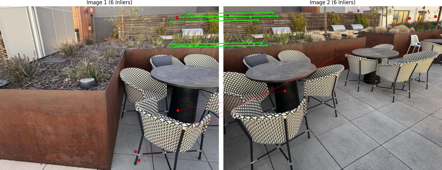
RANSAC Results
Below are the RANSAC results showing robust homography computation:
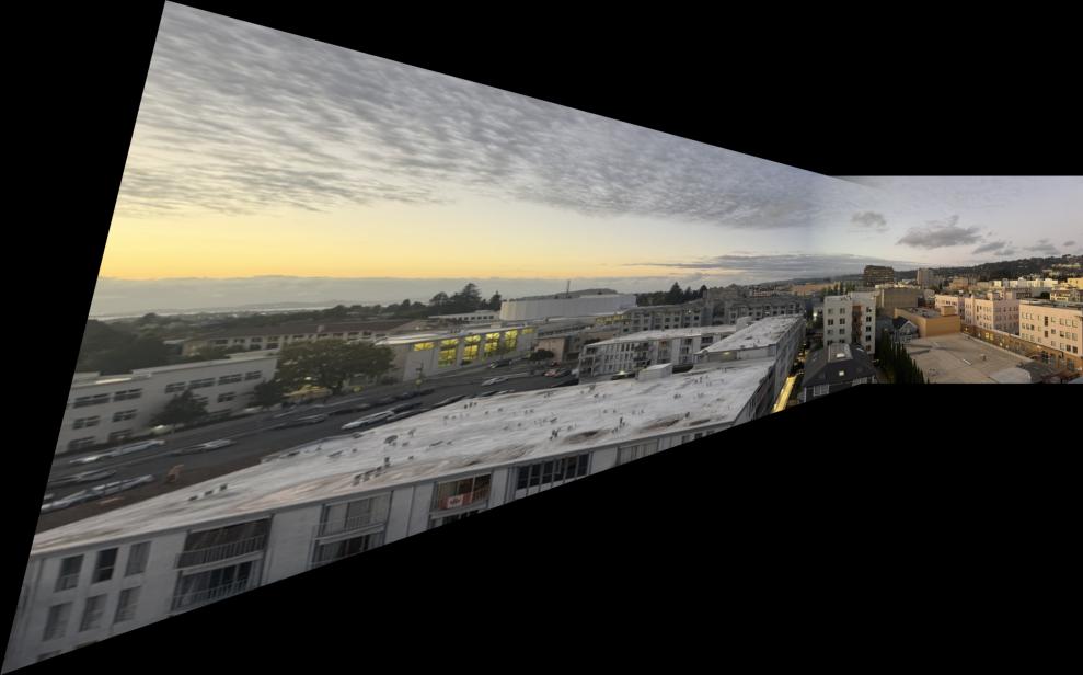
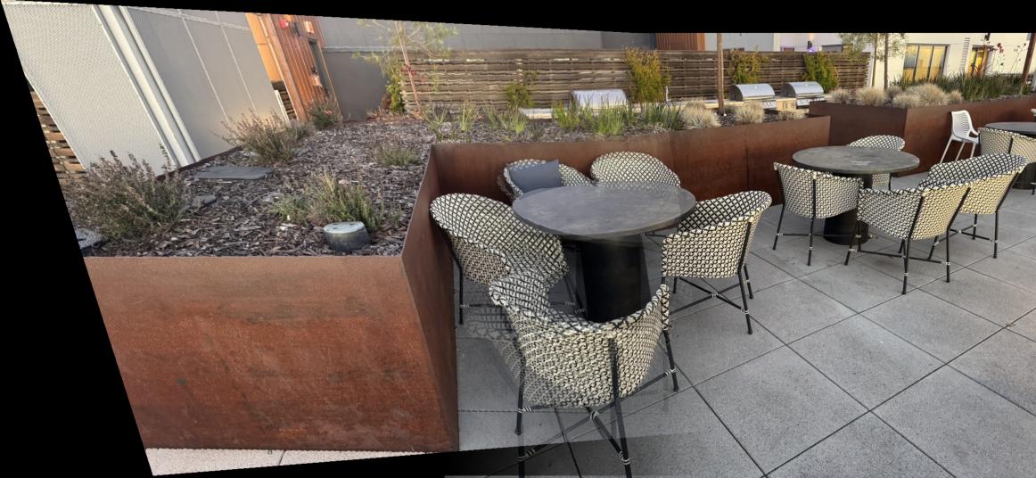
Automatic Mosaic Creation
Using the automatically detected and matched features with RANSAC, I created mosaics without manual point selection. The system computes homographies from the matched features and applies the same warping and blending techniques from Part A.
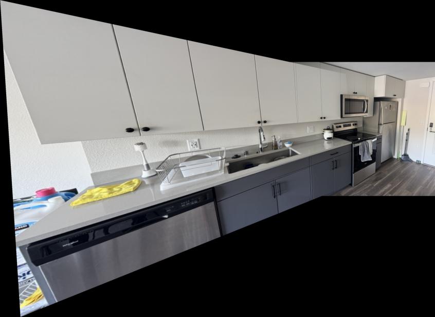
Comparison: Manual vs Automatic Stitching
Below are comparisons between manually stitched mosaics (from Part A) and automatically stitched mosaics (from Part B):
I learned that many of the hyperparameters had to be fine-tuned for each unique mosaic. That is because the automatic corner detection sometimes detects corners too close to each other, which means the alignment is not very diverse. Unlike the manual approach where I selected points diversely across the image, the automatic system can cluster features in certain regions.
Therefore, I had to adjust the Harris corner detection min_distance to be wider for some images, and the RANSAC epsilon sometimes also needed to be greater. An example where the pictures didn't work well for automatic stitching was the chair scene, as shown below. Sometimes, even after fine-tuning the hyperparameters, it did not align well. That is because there actually are not enough diverse corners shown in both images. All the diverse corners get filtered out by the algorithm, leaving only corners that are too similar or clustered in certain regions, which doesn't provide enough geometric diversity for robust homography estimation.
Project Summary
This project successfully implemented two complementary approaches to image mosaicing and warping:
Part A: Manual Image Warping and Mosaicing
- Homography Recovery: Computed 3x3 homography matrices from manually selected point correspondences
- Image Warping: Implemented inverse warping with both nearest-neighbor and bilinear interpolation
- Mosaic Creation: Blended multiple warped images into seamless panoramas using alpha blending
- Results: Successfully created high-quality mosaics for bay, chairs, downtown, and sink scenes
Part B: Automatic Feature Detection and Matching
- Harris Corner Detection: Implemented corner detection with adaptive non-maximum suppression (ANMS)
- Feature Descriptors: Extracted normalized 8x8 patch descriptors around detected corners
- Feature Matching: Matched features using SSD distance with ratio test for robustness
- RANSAC Homography: Computed robust homographies using 4-point RANSAC to handle outliers
- Results: Created automatic mosaics comparable in quality to manual stitching