proj4/
Neural Radiance Fields!
Overview
This project explores Neural Radiance Fields (NeRF), a cutting-edge technique for 3D scene representation and view synthesis. We implement neural networks that learn implicit representations of 3D scenes from multi-view images, enabling photorealistic view synthesis. The project spans from 2D neural fields to full 3D NeRF implementation, including camera calibration, volume rendering, and training on both synthetic and real-world data.
Part 0: Camera Calibration and 3D Scanning
For this section, I calibrated my camera using ArUco tags and captured multi-view images of a chosen object. The calibration process involved capturing 30-50 images of ArUco calibration tags, extracting corner coordinates, and using OpenCV's camera calibration to compute intrinsic parameters and distortion coefficients.
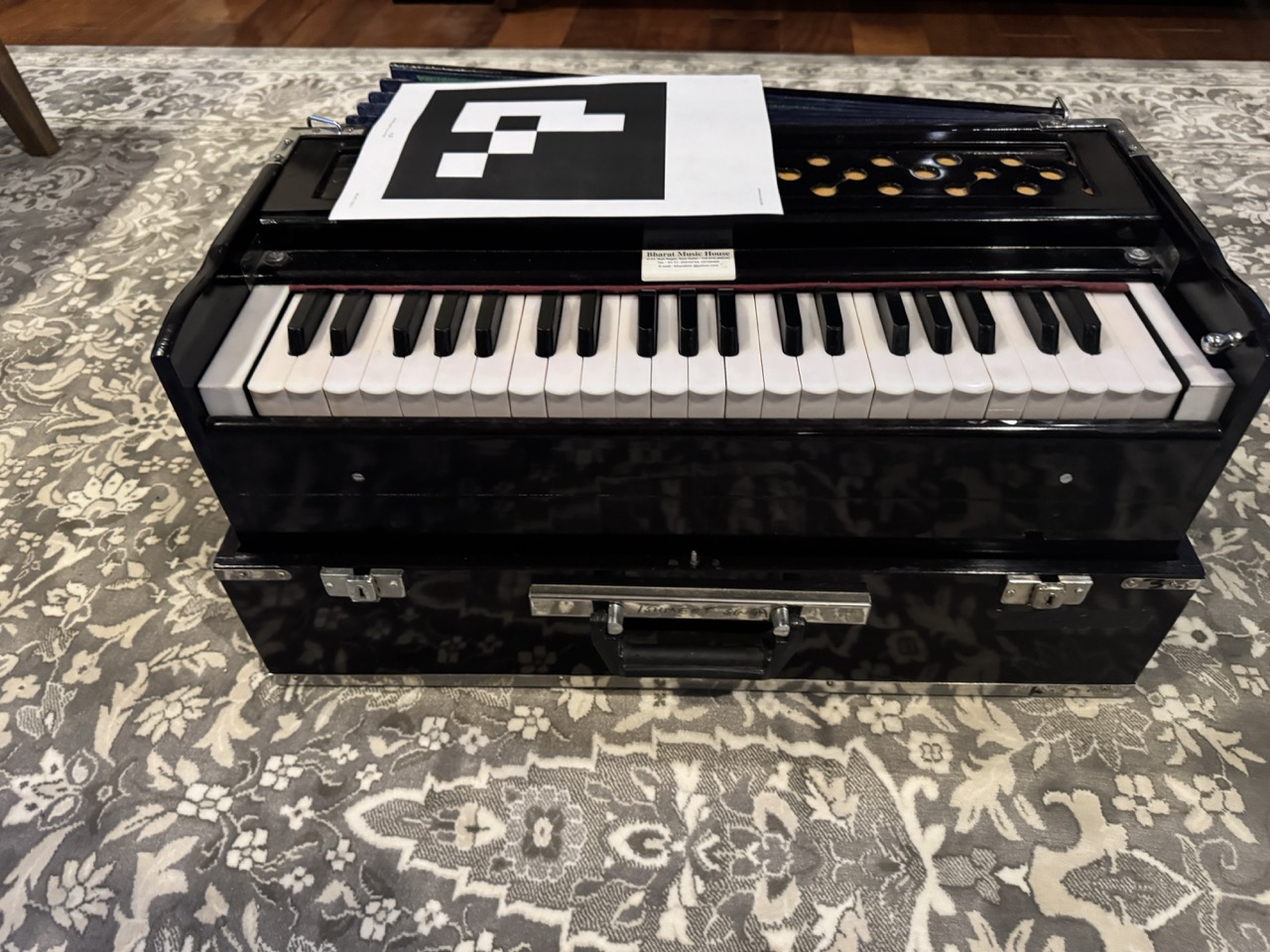
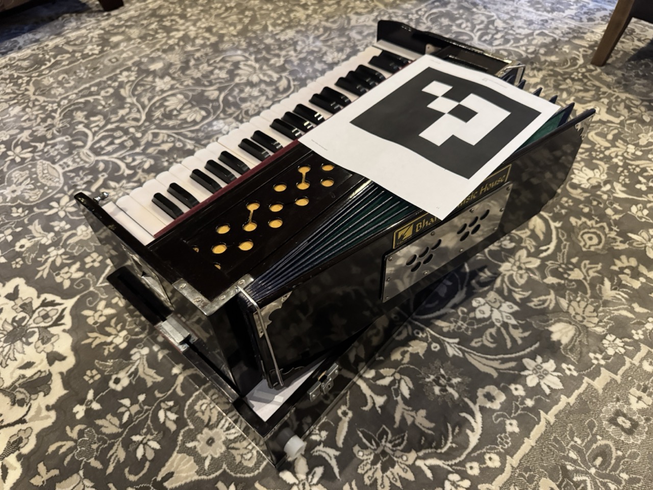
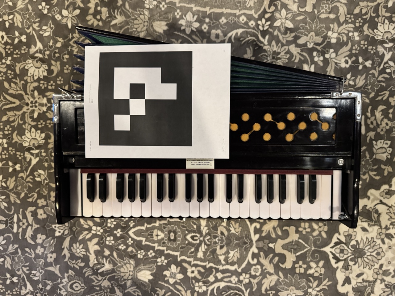
After calibration, I captured images of my chosen object (a small figurine) alongside a single ArUco tag, then used the calibrated camera parameters to estimate camera poses via solvePnP. The final step involved undistorting images and packaging everything into a dataset format compatible with NeRF training.
Sample Images from Data Capture
Examples of captured images showing the object alongside the ArUco tag for pose estimation:
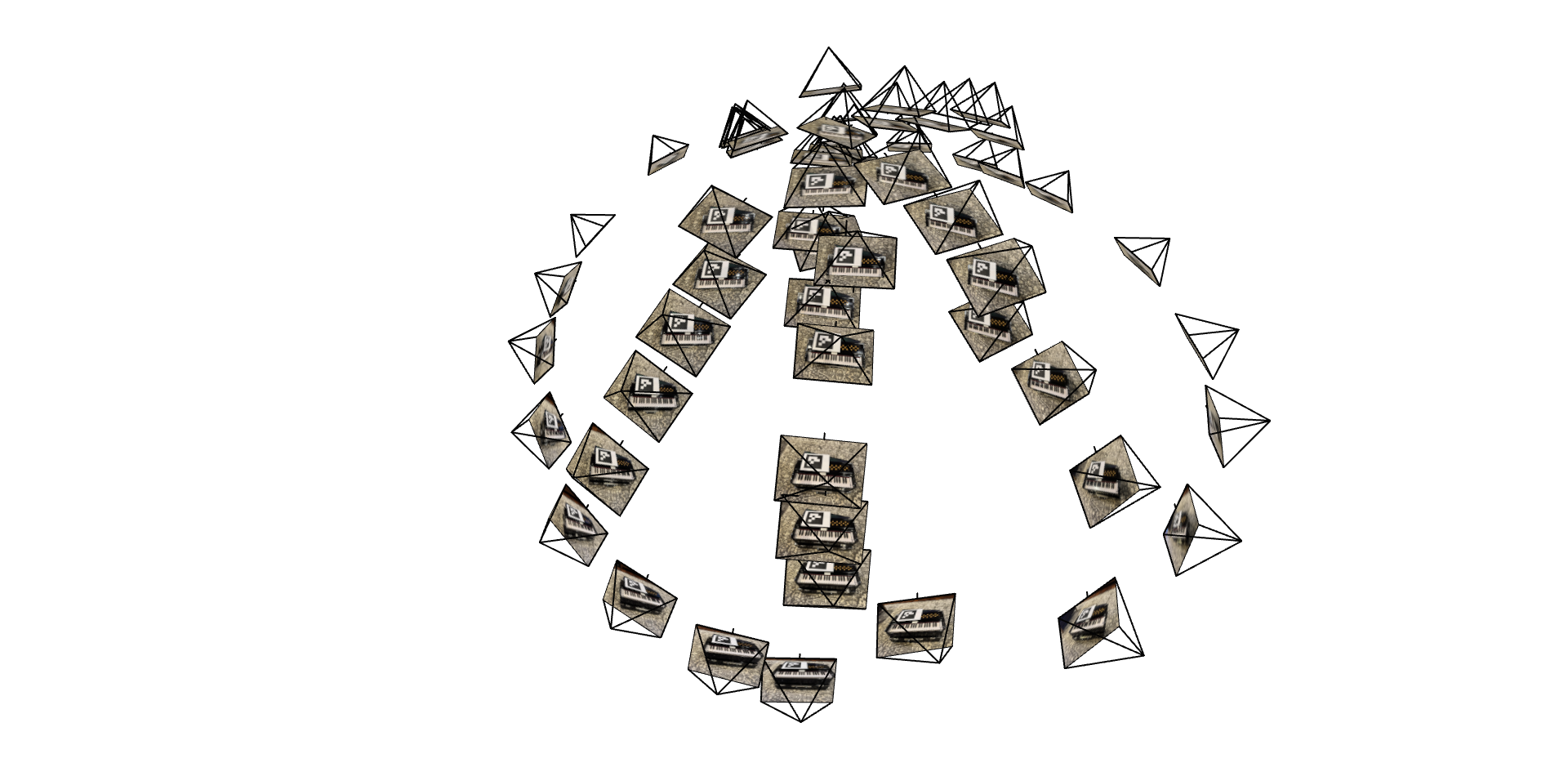
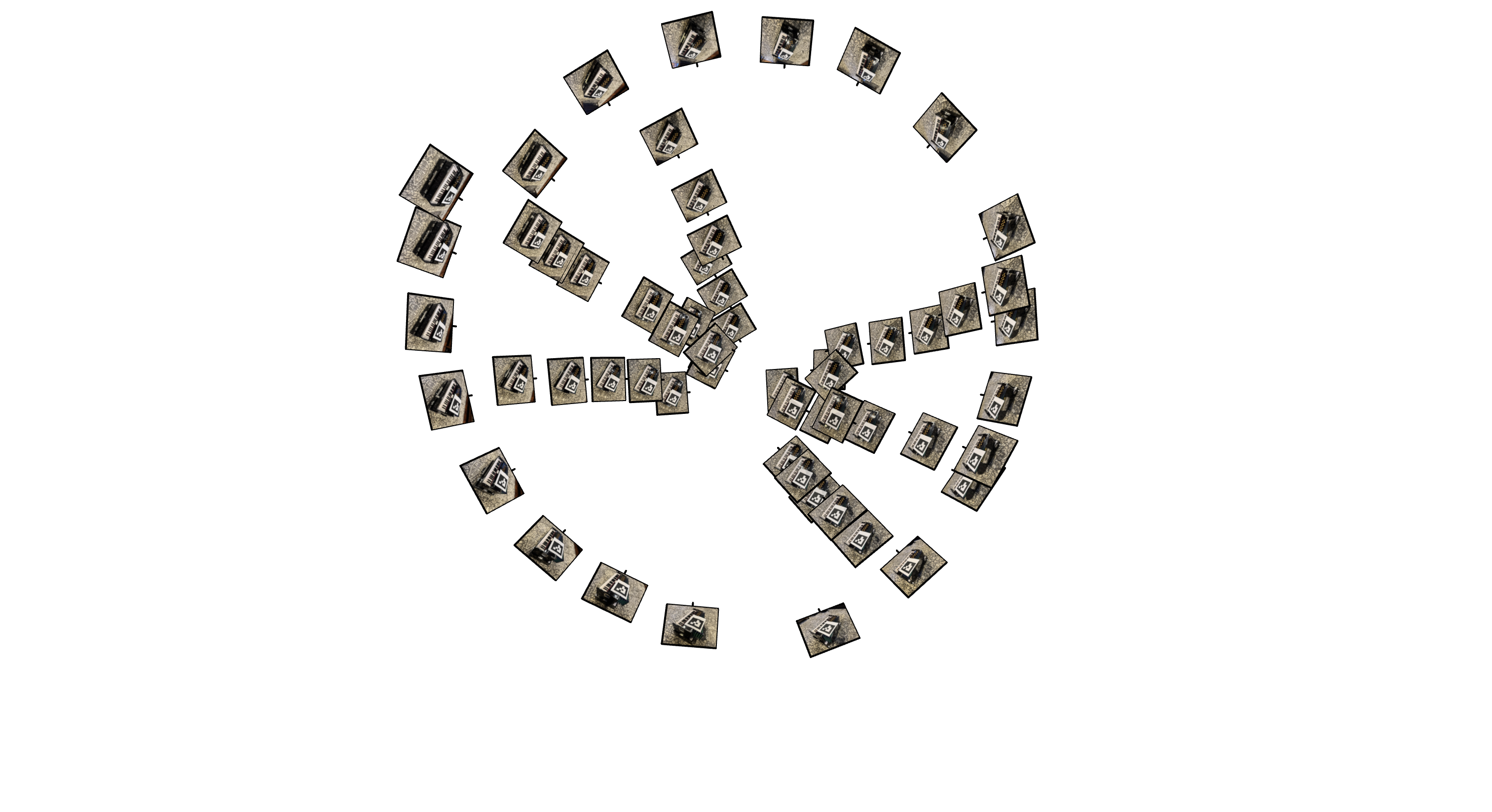
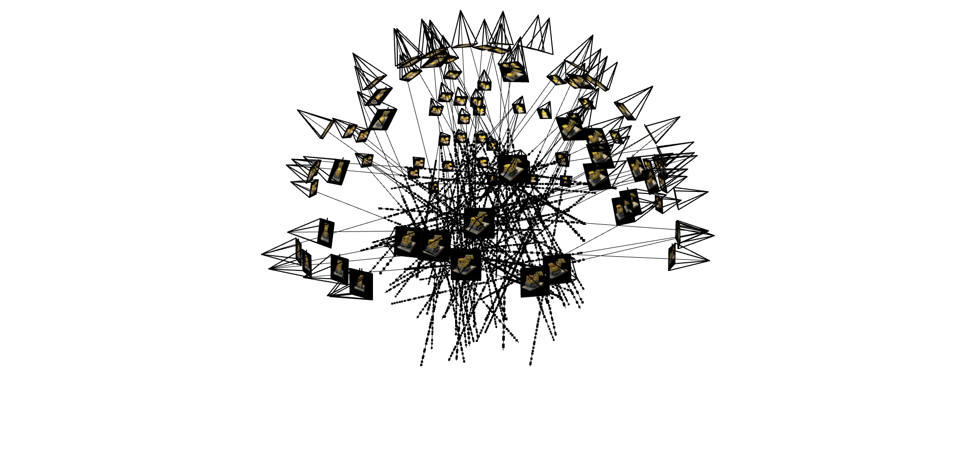
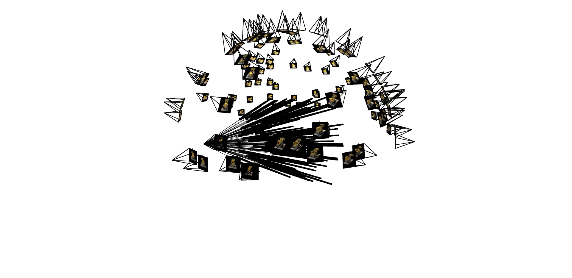
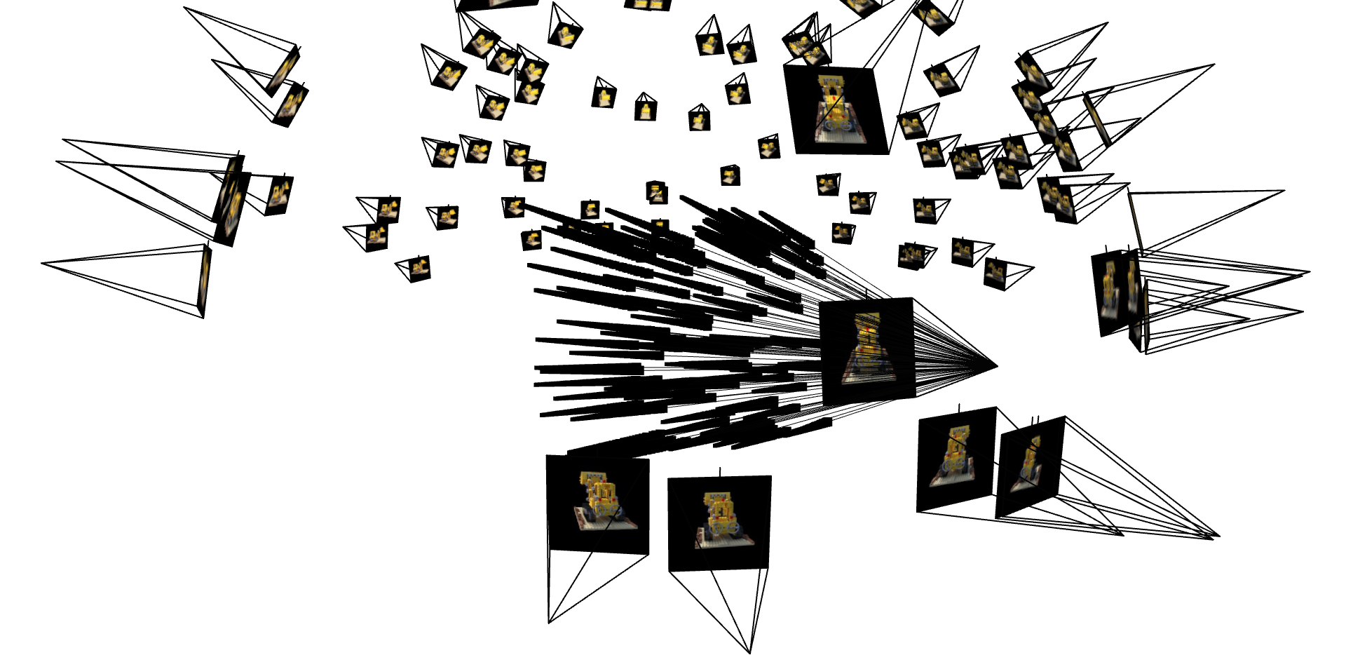
Camera Frustum Visualizations
Screenshots of the camera frustums visualization in Viser, showing the estimated camera poses:
Part 1: 2D Neural Field
Before implementing 3D NeRF, I started with a simpler 2D version to understand the fundamentals. I created a Multilayer Perceptron (MLP) with Sinusoidal Positional Encoding that takes 2D pixel coordinates as input and outputs RGB color values. The network was trained to fit entire images by optimizing pixel-wise color predictions.
2D Neural Field Architecture
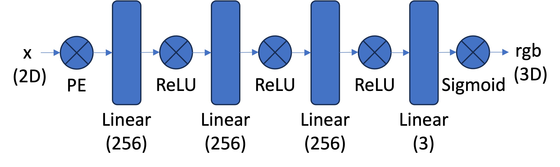
Network Architecture Details:
- Number of Layers: 4-layer MLP (3 hidden layers + output layer)
- Width: 256 hidden units per layer
- Input Dimension: $L \times 2 \times 2 + 2 = 42$ for $L=10$ positional encoding
- Output Dimension: 3 (RGB color values)
- Activation Functions: ReLU for hidden layers, Sigmoid for output
- Positional Encoding: Sinusoidal PE with $L=10$ frequency levels
- Learning Rate: $1 \times 10^{-2}$ with Adam optimizer
- Batch Size: 10,000 pixels sampled per epoch
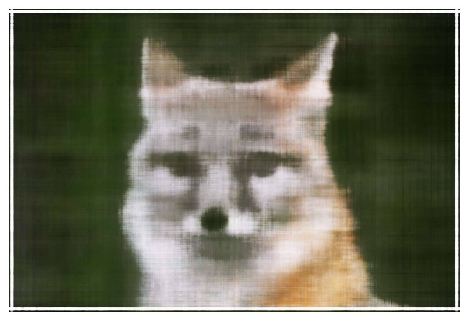
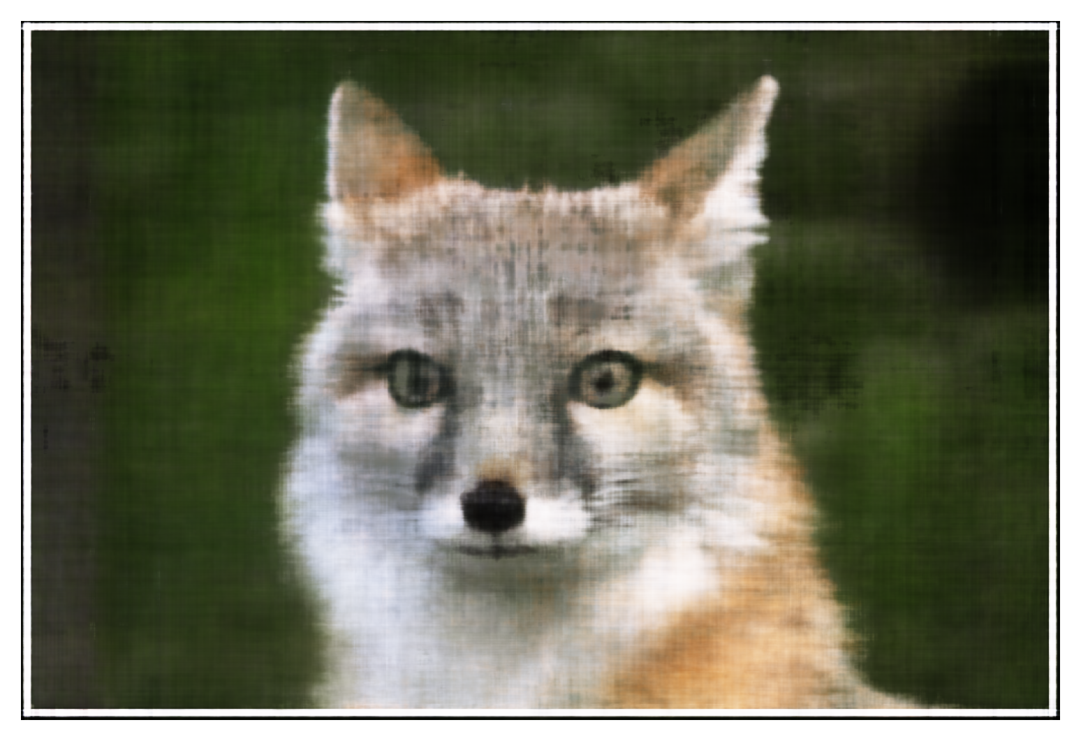
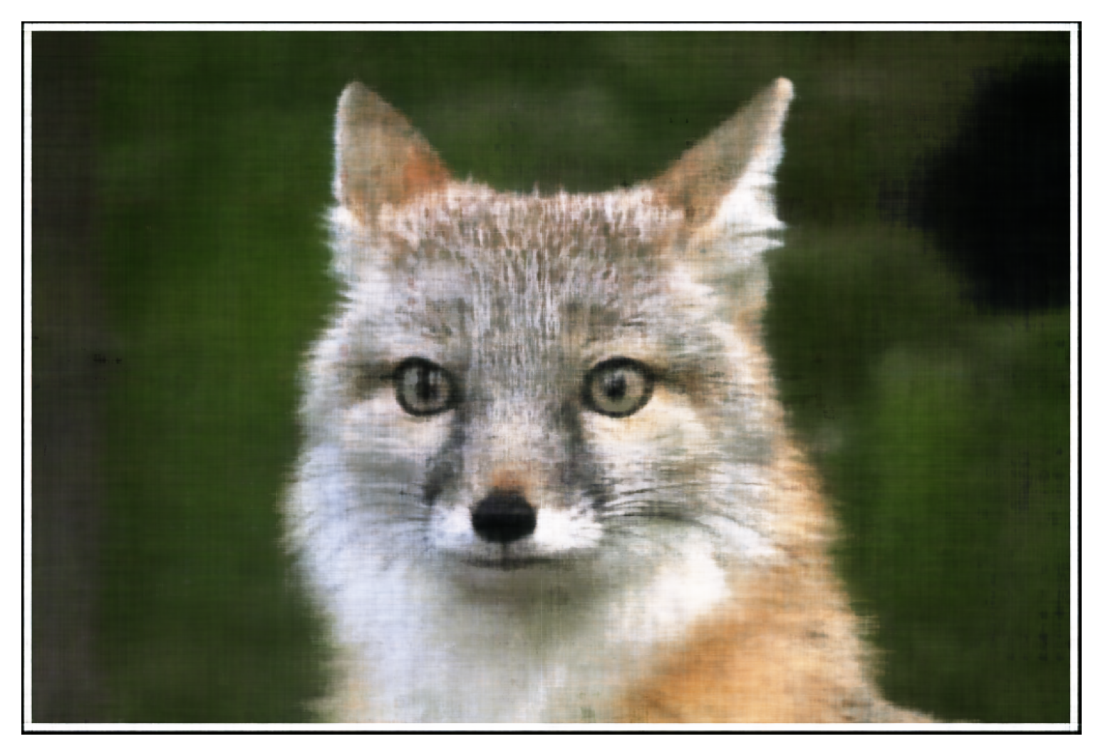
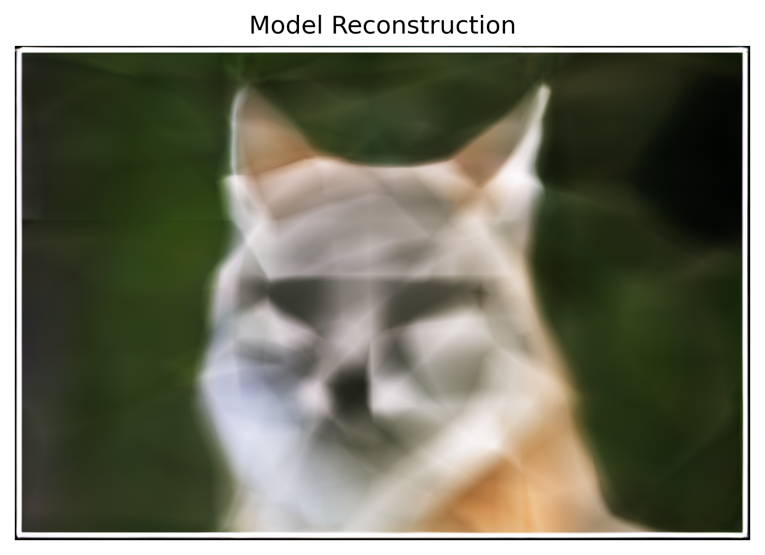
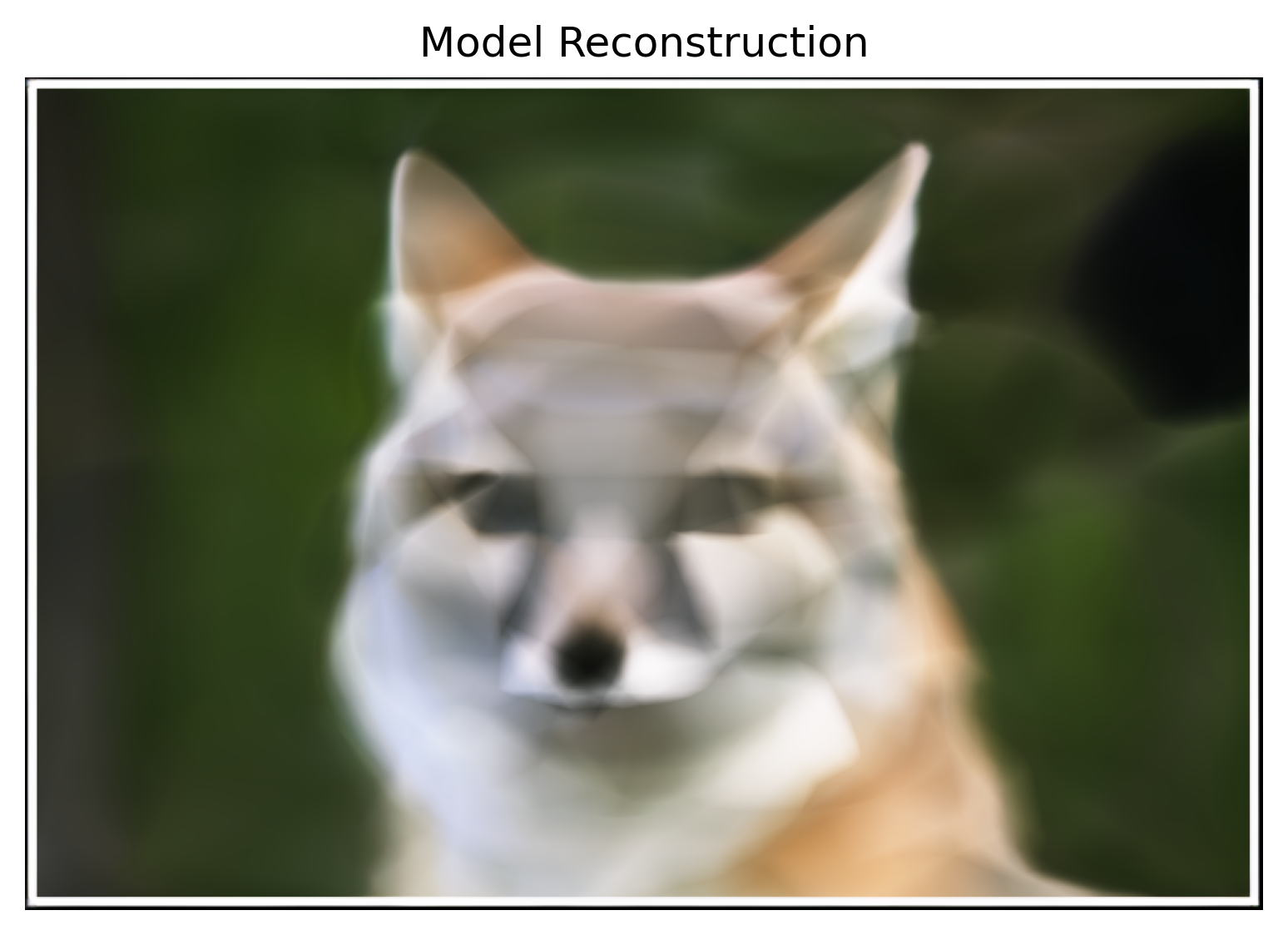
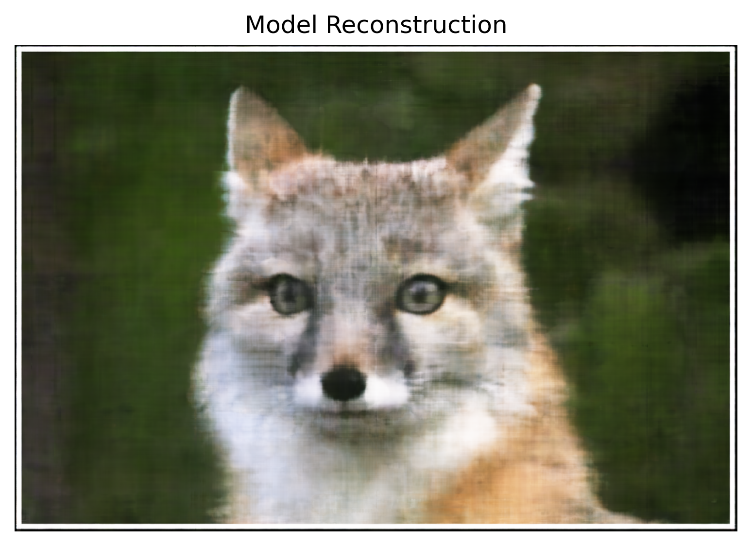
Training Progression
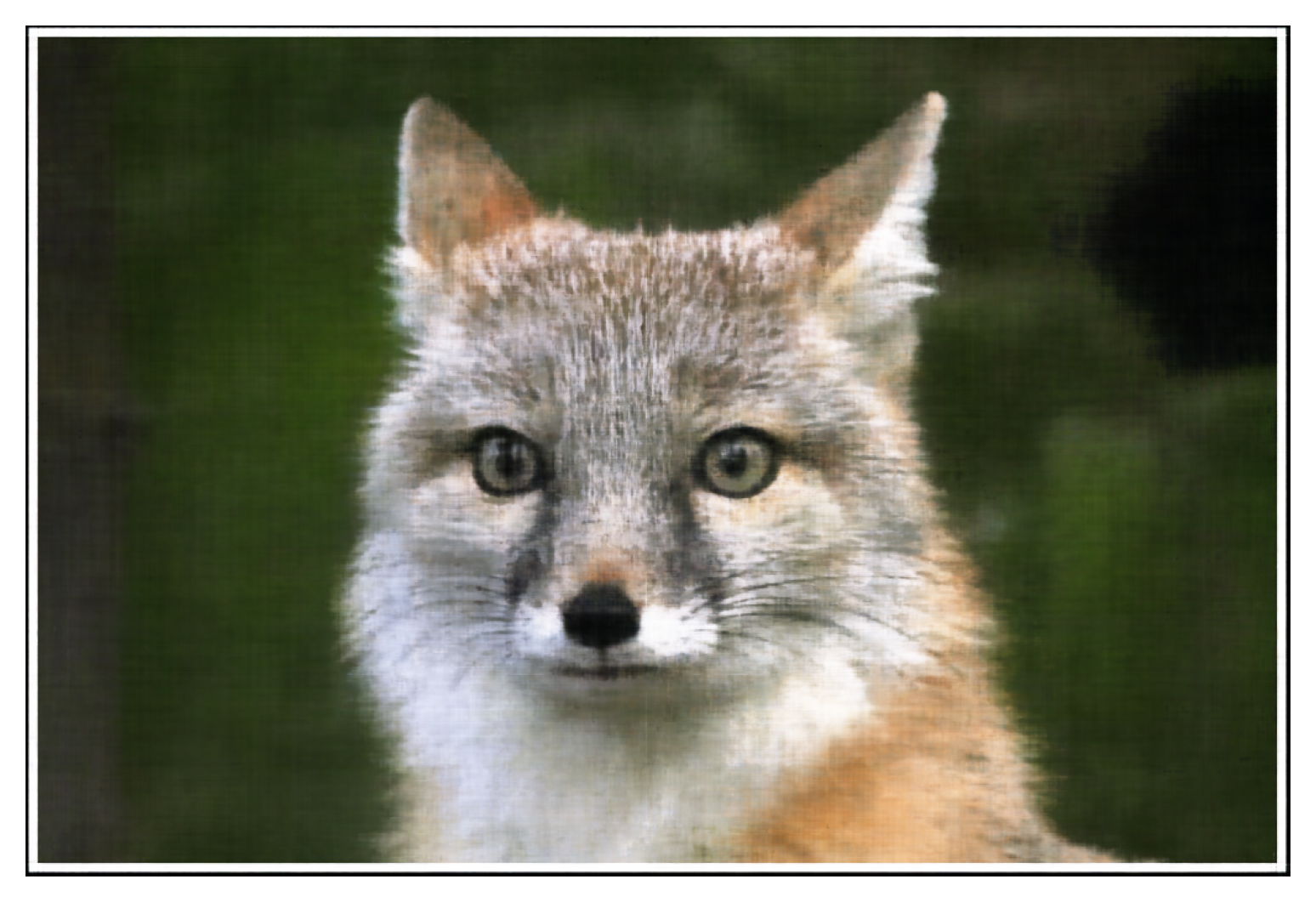
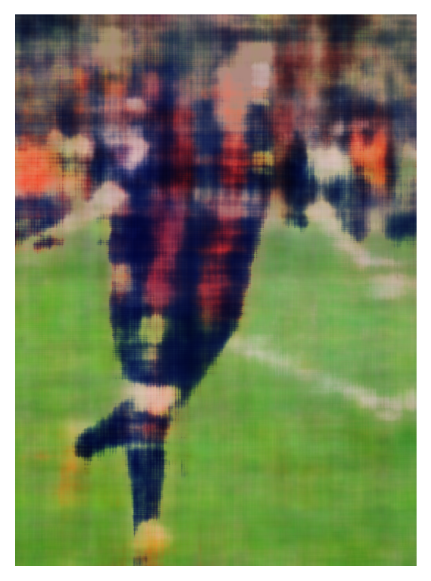
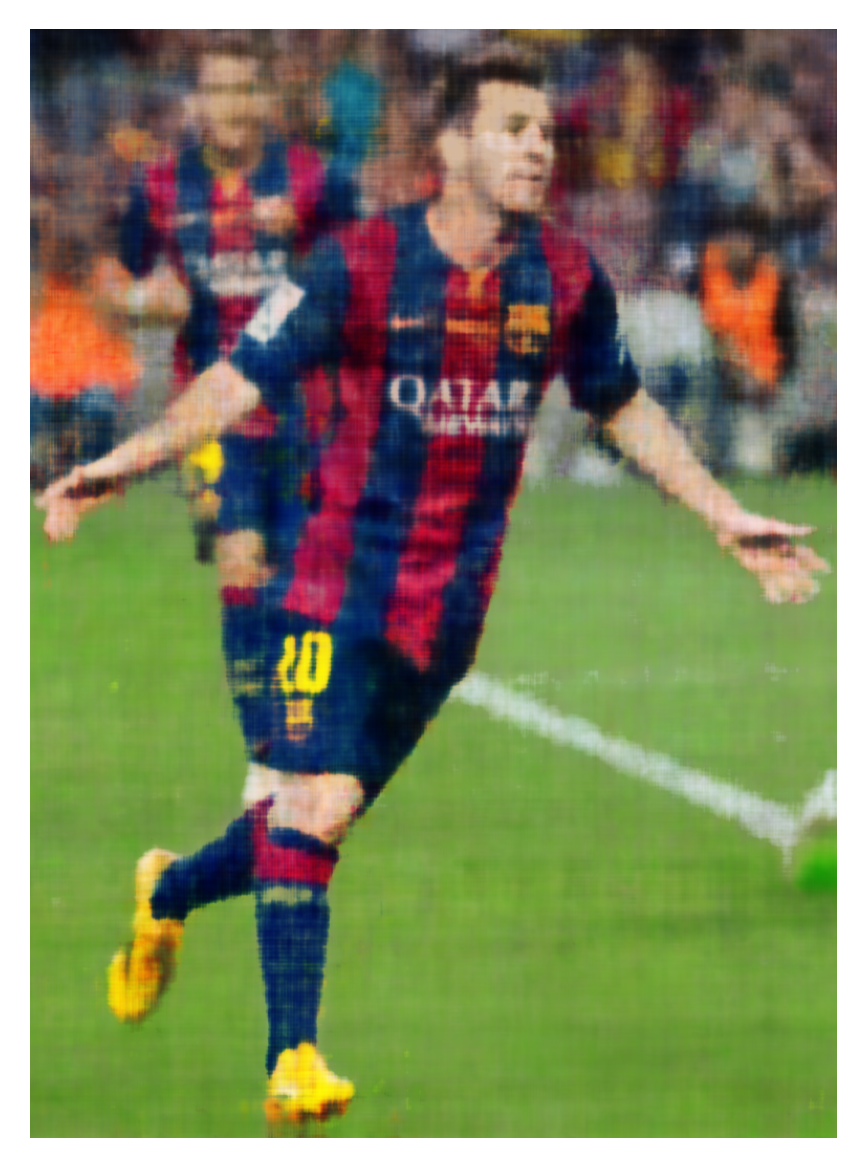
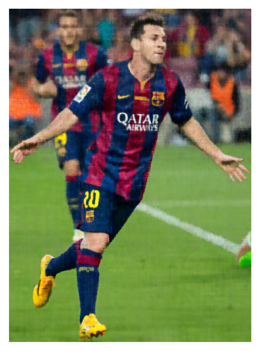
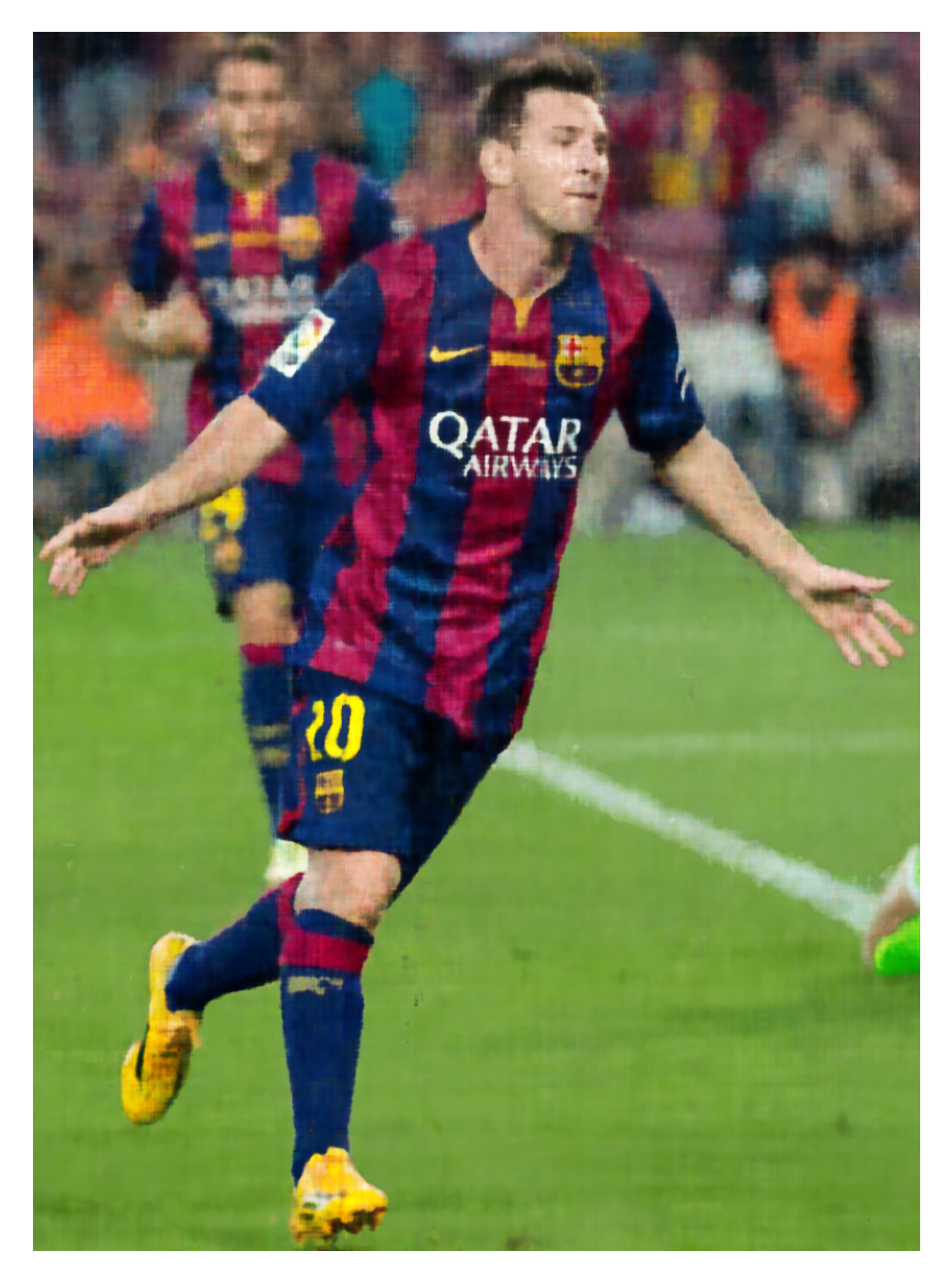
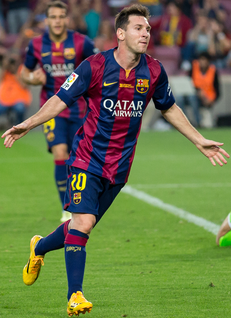
Below shows the training progression for both the provided fox image and my own Messi image:
Fox Image Training
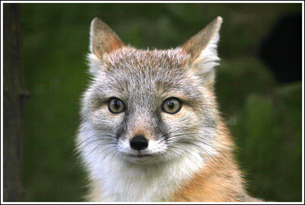
Messi Image Training
Hyperparameter Analysis
I experimented with different positional encoding frequencies (L) and network widths:

As expected, higher positional encoding frequencies ($L=10$) capture fine details better than lower frequencies ($L=2$). Similarly, wider networks (256 units) produce smoother reconstructions compared to narrower ones (64 units).
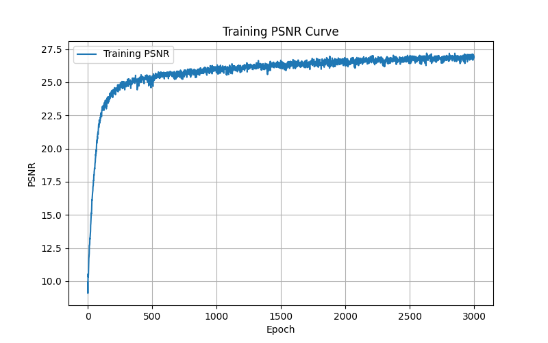
Training Metrics
Fox Image Training Curves
Messi Image Training Curves
Part 2: Neural Radiance Field from Multi-view Images
Building on the 2D neural field foundation, I implemented a full Neural Radiance Field that represents 3D scenes from multi-view images using inverse rendering from calibrated cameras.
Part 2.1: Create Rays from Cameras
I implemented three core coordinate transformations to generate camera rays. First, I used 4×4 transformation matrices to convert points from camera space to world coordinates: $\mathbf{x}_w = \mathbf{R} \mathbf{x}_c + \mathbf{t}$. Then I inverted the camera intrinsic matrix to convert pixel coordinates to 3D camera coordinates: $\mathbf{x}_c = K^{-1} \begin{bmatrix} u \\ v \\ 1 \end{bmatrix}$. Finally, I generated rays by computing the origin as the camera position $\mathbf{o} = \mathbf{t}$ and the direction as the normalized vector from camera center through each pixel.
Part 2.2: Sampling
I implemented random ray sampling from multi-view images, adding 0.5 to UV coordinates to sample from pixel centers rather than corners. For each ray, I uniformly sampled 64 points between near and far planes by dividing the ray into equal intervals. During training, I added random perturbations $t_i = t_i + \mathcal{U}(0, \Delta t)$ to sample positions to prevent overfitting and ensure the model explores all locations along each ray.
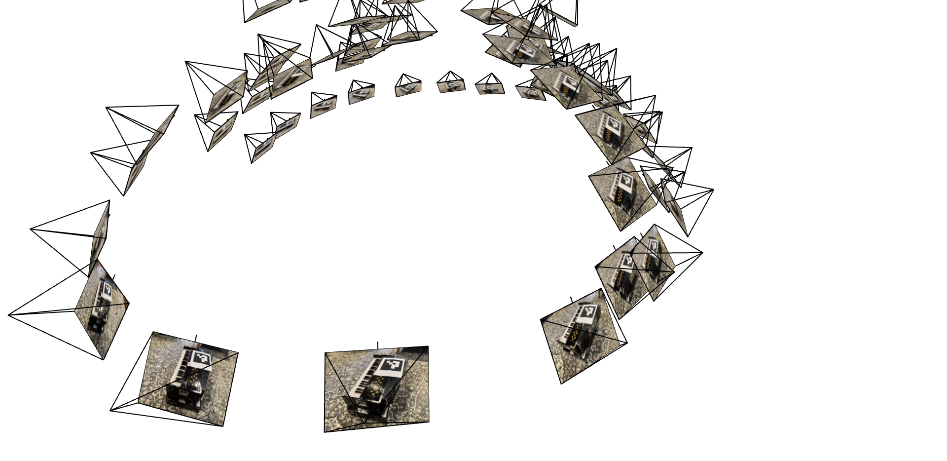
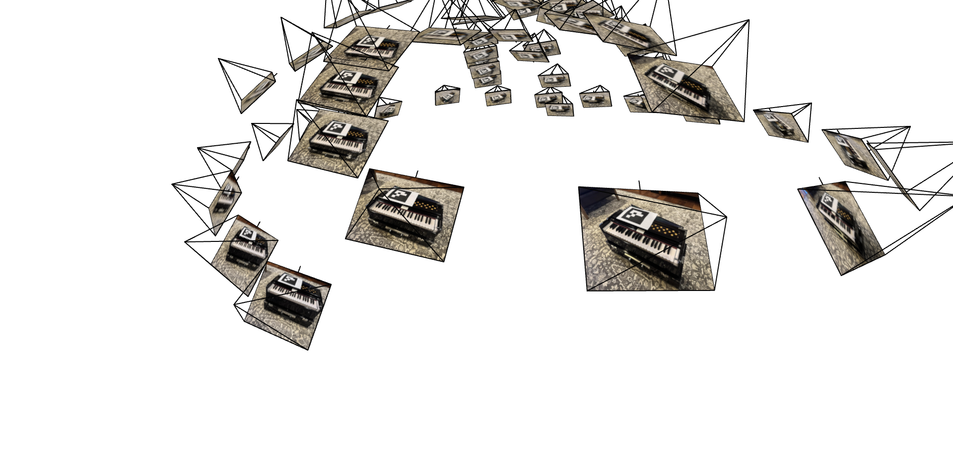
Part 2.3: Putting the Dataloading All Together
I created a unified $\texttt{RaysData}$ class that precomputes ray origins and directions for all training images, then efficiently samples 10,000 random rays per iteration. This dataloader returns ray origins, directions, and corresponding ground truth RGB colors for batch training. I verified the implementation by visualizing camera frustums, rays, and 3D sample points using Viser.
Part 2.4: Neural Radiance Field
I built an 8-layer MLP that takes positionally-encoded 3D coordinates ($L=10$) and view directions ($L=4$) as input. The network uses skip connections at layer 5 and has separate heads for density prediction (with ReLU) and view-dependent color prediction (with Sigmoid). There's also a skip connection for the RGB branch where the view directions ($\mathbf{r}_d$) are concatenated at the second RGB fully connected layer. This architecture allows the model to capture both geometric structure and view-dependent appearance effects.
3D Neural Radiance Field Architecture

Part 2.5: Volume Rendering
I implemented the discrete volume rendering equation to composite colors and densities along rays into final pixel colors: $C(\mathbf{r}) = \sum_{i=1}^{N} T_i \alpha_i \mathbf{c}_i$. The function computes alpha values $\alpha_i = 1 - \exp(-\sigma_i \delta_i)$ and transmittance $T_i = \exp(-\sum_{j=1}^{i-1} \sigma_j \delta_j)$ using cumulative sums for proper alpha compositing. My implementation passed the provided torch.allclose() test, ensuring correct mathematical computation of the rendering integral.
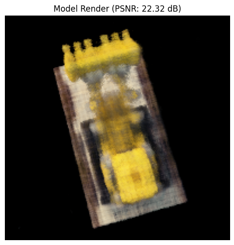
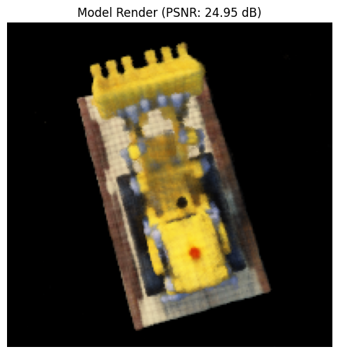
Training Progression
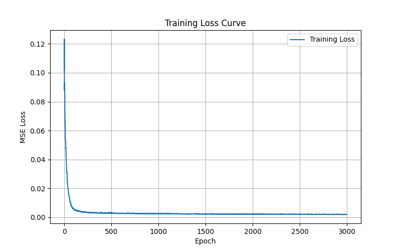
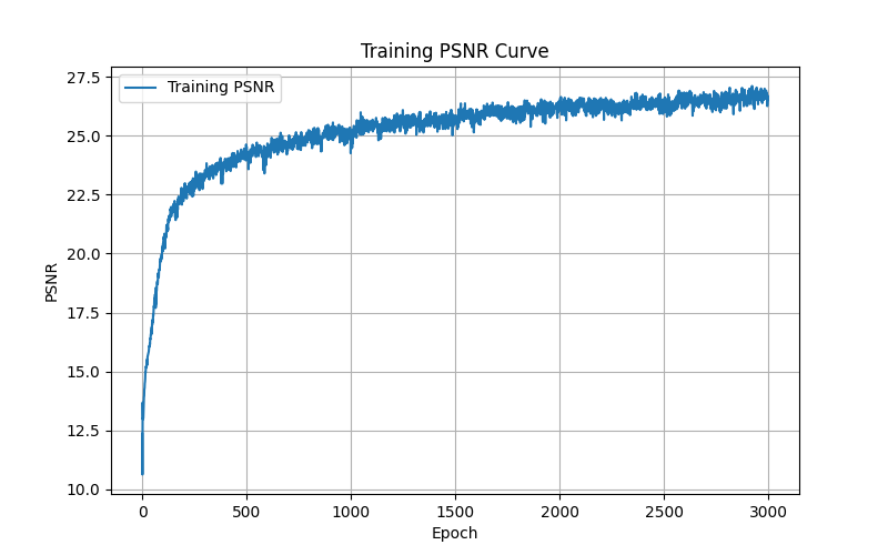
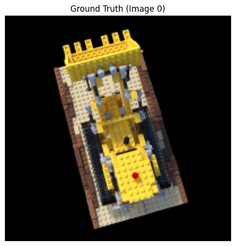
Training progression showing the NeRF learning to represent the Lego scene. The model was trained for 2000 epochs using Adam optimizer with learning rate $5 \times 10^{-4}$, sampling 10,000 rays per iteration and 64 points per ray. Near and far planes were set to $z_{\text{near}}=2.0$ and $z_{\text{far}}=6.0$ respectively. The network uses positional encoding with $L=10$ frequencies for 3D coordinates and $L=4$ frequencies for view directions, with 256 hidden units per layer.

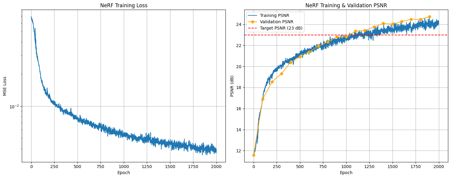
Training Metrics
Spherical Rendering
Spherical rendering of the Lego scene:
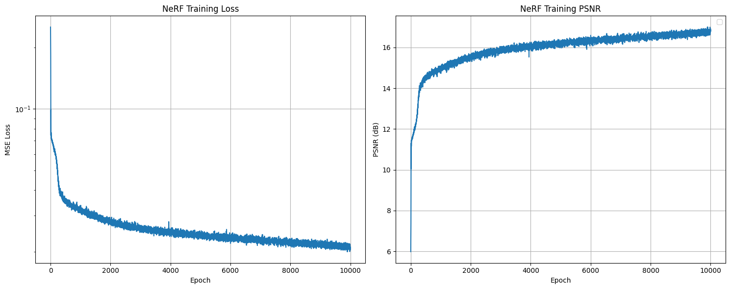
Part 2.6: Training NeRF on Own Data
Using the dataset I created in Part 0, I trained a NeRF on my own captured object. This involved adapting the network hyperparameters for real-world data, adjusting the near/far sampling bounds, and fine-tuning the training process to handle the challenges of real camera data compared to the synthetic Lego scene.
Hyperparameters for Real Data
Training Configuration:
- Near/Far Bounds: $z_{\text{near}}=0.02$, $z_{\text{far}}=0.5$ for close-up object capture
- Camera Intrinsics: Used actual calibrated K matrix from ArUco calibration
- Samples per Ray: 64 samples with denser sampling due to smaller depth range
- Learning Rate: $5 \times 10^{-4}$ with Adam optimizer
- Training Duration: 10,000 epochs for proper convergence
- Batch Size: 10,000 rays per iteration
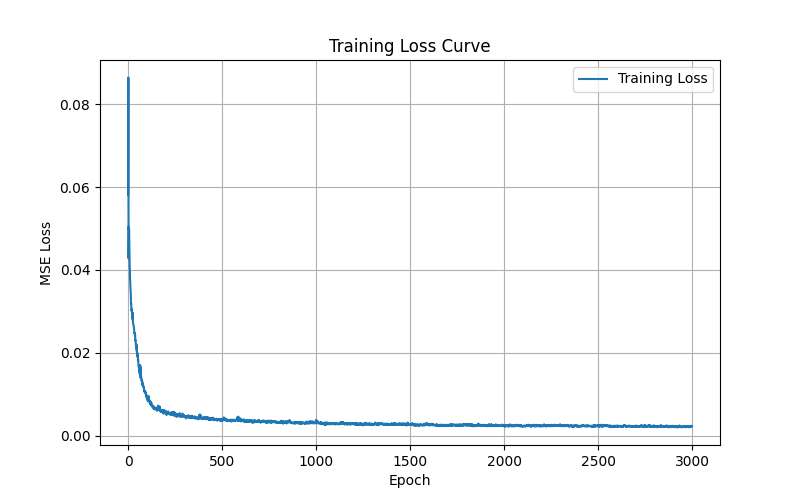
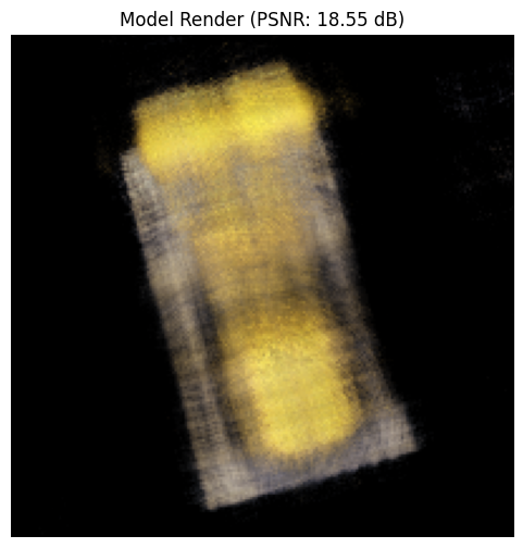
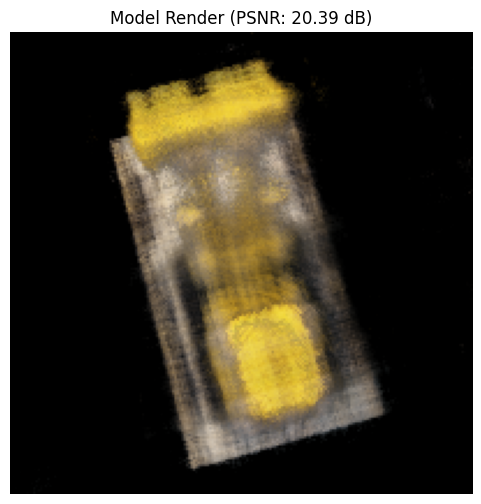
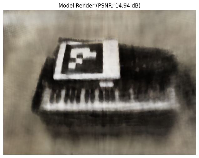
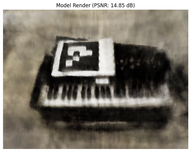
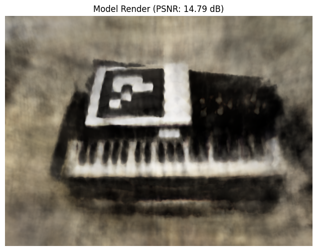
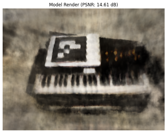
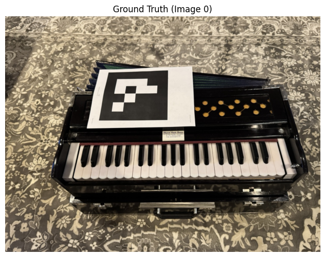
Training Progression
Training progression showing the NeRF learning to represent my captured object. We can observe significant improvements in fine details as training progresses - the harmonium keys become increasingly well-defined and the yellow holes on the top near the ArUco tag become more visible and accurately rendered:
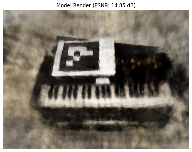
Training Metrics
Spherical Rendering
Circular orbit rendering of my captured object: