proj5/
Diffusion Models!
Overview
This project explores diffusion models, a powerful class of generative models that learn to reverse a gradual noising process to generate high-quality images from text prompts. We work with the DeepFloyd IF model, implementing diffusion sampling loops and experimenting with various text-to-image generation tasks.
Part A: The Power of Diffusion Models!
Part 0: Setup
Generated Prompt Embeddings
I generated embeddings for the following text prompts, exploring a variety of subjects and artistic styles:
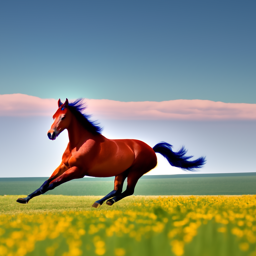
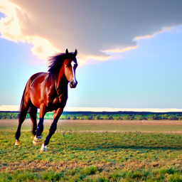
- 'a photo of a horse running through a meadow'
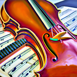
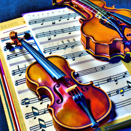
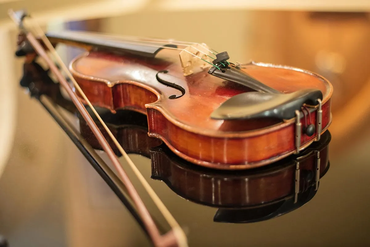
- 'an oil painting of a violin resting on sheet music'
- 'a high quality picture of a dinosaur in a forest'
- 'a photo of the Golden Temple at sunrise'
- 'a still life painting of pumpkins on a wooden table'
- 'a neon sign that says OPEN glowing in the dark'
- 'a high quality photo of a Porsche on a mountain road'
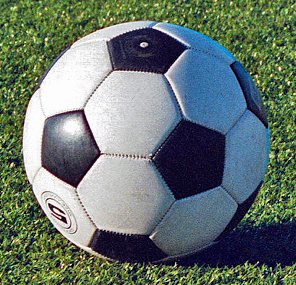
- 'a photo of a soccer ball on a wet field at night'
- 'a high quality image'
- 'a single lone tree in a field'
- 'a king without a crown'
- 'a crown sitting on a table'
- 'a piece of sushi on a plate with chopsticks'
- 'a roll of toilet paper'
Selected Images and Analysis
From my prompt collection, I selected the following three for image generation and analysis:


Reflection on Model Output Quality
The DeepFloyd model demonstrates impressive capability in understanding and translating text descriptions into coherent visual representations:
- Horse running through meadow: The model successfully captures the motion and natural setting, showing good understanding of spatial relationships and movement dynamics.
- Violin on sheet music: The artistic prompt resulted in a composition that conveys the classical, refined aesthetic requested. The model interprets "oil painting" style appropriately.
- Dinosaur in forest: This fantastical prompt showcases the model's ability to combine elements that don't typically coexist in reality, creating a believable prehistoric scene.
All images were generated using the same random seed (100) for consistency. The model shows strong semantic understanding and generates visually coherent results that align well with the textual descriptions.
Part 1: Sampling Loops
1.1 Implementing the Forward Process
The forward process adds noise to a clean image progressively. I implemented this using the equation:
where $\epsilon$ is random noise sampled from a standard normal distribution $\mathcal{N}(0, I)$.
Here's the Berkeley Campanile at different noise levels (timesteps):


1.2 Classical Denoising
I attempted to denoise the noisy Campanile images using classical Gaussian blur filtering. As expected, this approach struggles significantly with higher noise levels and doesn't produce satisfactory results.


1.3 One-Step Denoising
Using the pretrained DeepFloyd UNet, I implemented one-step denoising. The model estimates the noise in the image and removes it to recover an approximation of the original clean image. This approach works significantly better than Gaussian blur, especially at lower noise levels.


1.4 Iterative Denoising
I implemented iterative denoising which removes noise over multiple steps, producing much higher quality results than single-step denoising.
Here's the progressive denoising process shown every 5th step:


Final comparison of different denoising approaches:


1.5 Diffusion Model Sampling
Using the iterative denoising function starting from pure noise (i_start = 0), I generated 5 samples with the prompt "a high quality photo". The results demonstrate the model's ability to generate diverse images from random noise.


1.6 Classifier-Free Guidance (CFG)
To improve image quality, I implemented Classifier-Free Guidance with $\gamma = 7$. This technique computes both conditional and unconditional noise estimates, then combines them to produce higher quality images.


1.7 Image-to-image Translation
Following the SDEdit algorithm, I added noise to the original Campanile image and then denoised it using the prompt "a high quality photo". Different noise levels create different degrees of editing, with higher noise levels allowing for more dramatic changes.


Results on my own test images:
Soccer Ball Image


Violin Image


1.7.1 Editing Hand-Drawn and Web Images
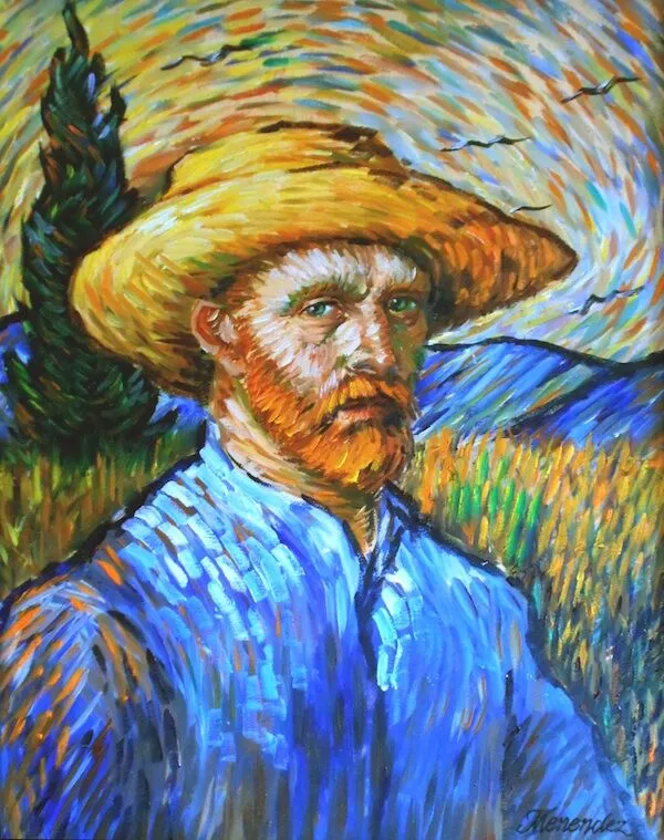
This procedure works particularly well when starting with non-realistic images and projecting them onto the natural image manifold. I experimented with both web images and hand-drawn sketches.
Painting Web Image


Hand-Drawn Image 1
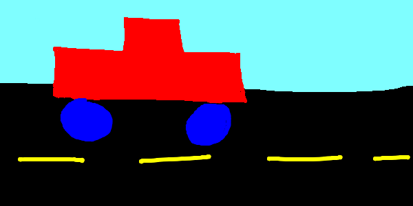


Hand-Drawn Image 2


1.7.2 Inpainting
Following the RePaint algorithm, I implemented inpainting by running the diffusion denoising loop while forcing pixels outside the edit mask to match the original image (with appropriate noise added for each timestep).


Billboard Inpainting


Tree Inpainting


1.7.3 Text-Conditional Image-to-image Translation
Similar to SDEdit but now guided by specific text prompts. This allows for more controlled edits that not only project onto the natural image manifold but also incorporate semantic guidance from the text prompt.
Campanile → Golden Temple at Sunrise


Soccer Ball → Golden Temple at Sunrise


Violin → Golden Temple at Sunrise


1.8 Visual Anagrams
Visual anagrams are optical illusions created using diffusion models that show different images when viewed right-side up versus upside down. I implemented this by averaging noise estimates from two different text prompts - one for the normal orientation and one for the flipped image.
Campfire People ↔ Old Man


Horse ↔ Dinosaur


Pumpkins ↔ Porsche


1.9 Hybrid Images
Following Factorized Diffusion, I created hybrid images by combining low frequencies from one noise estimate with high frequencies from another. This technique creates images that appear different when viewed from various distances or when the viewing conditions change.

High-pass: "A roll of toilet paper"

High-pass: "A single lone tree in a field"
Part B: Flow Matching from Scratch!
In this part, we'll train our own flow matching model on MNIST from scratch. Flow matching is a powerful technique for generative modeling that learns to map noise to data through a continuous flow. We'll implement and train a UNet to perform this transformation iteratively.
Part 1: Training a Single-Step Denoising UNet
1.1 Implementing the UNet
I implemented a UNet architecture for denoising noisy MNIST digits. The UNet consists of downsampling and upsampling blocks with skip connections, designed to map noisy images back to clean images in a single step.
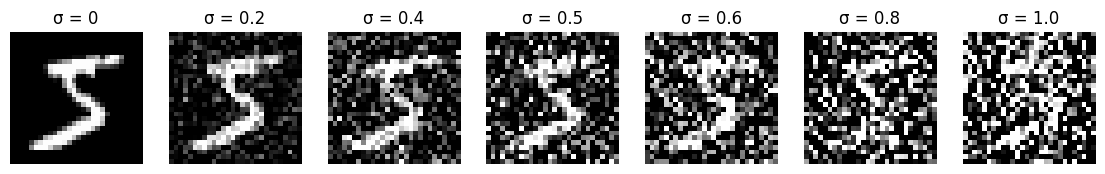
1.2 Denoising Process Visualization
To understand how noise affects the input images, I visualized the noising process using $\sigma \in \{0, 0.2, 0.4, 0.5, 0.6, 0.8, 1\}$. This shows how different noise levels progressively corrupt the original MNIST digits.
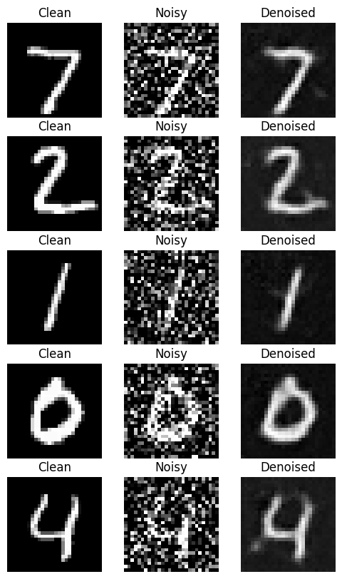
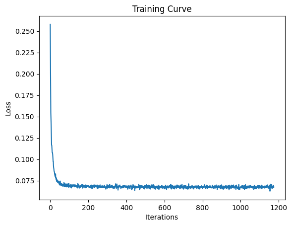
1.2.1 Training Results
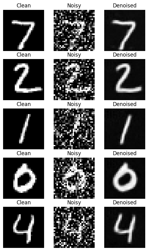
I trained the denoising UNet for 5 epochs using the MNIST dataset with $\sigma = 0.5$. The model learns to map noisy images $\tilde{x}$ back to clean images $x$. Here are the results after 1 and 5 epochs of training:
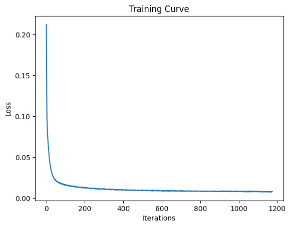
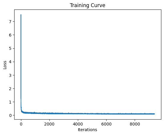
Training Loss Curve
1.2.2 Out-of-Distribution Testing
I tested the trained denoiser (which was trained on σ = 0.5) on different noise levels that it hadn't seen during training. This evaluates the model's generalization to different noise conditions.
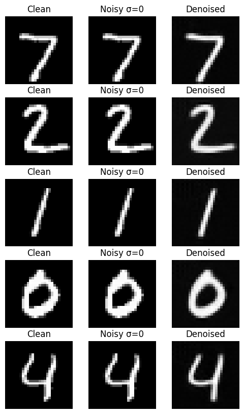
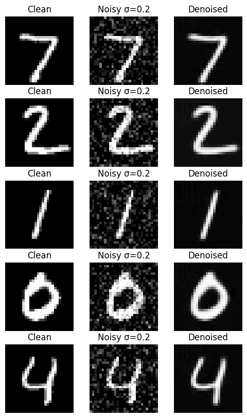
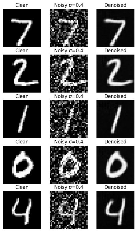
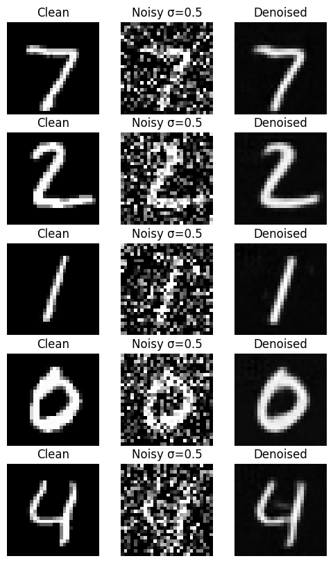
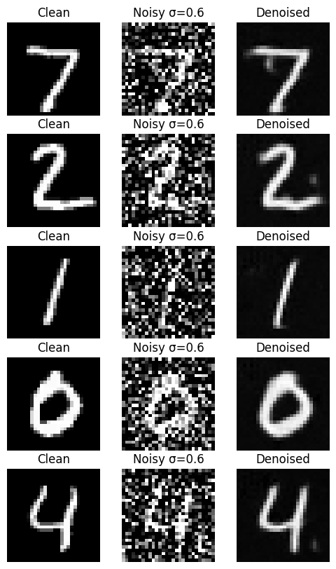
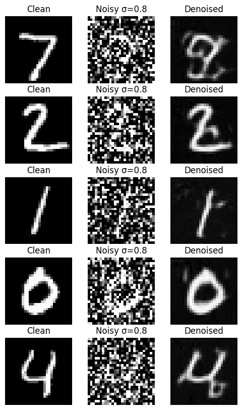
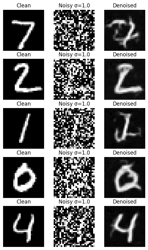
The results show that the model performs best at the noise level it was trained on (σ = 0.5) and levels below that, with decreasing quality as we move upwards from this training condition. At very high noise levels (σ = 1.0), the model struggles significantly.
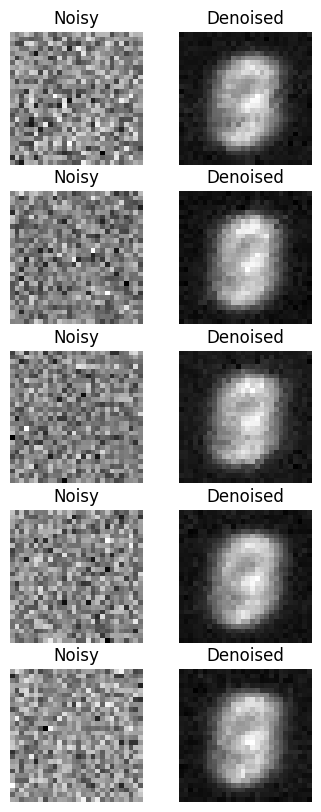
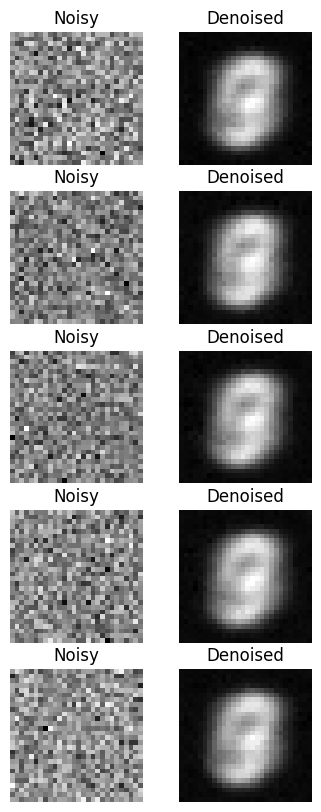
1.2.3 Denoising Pure Noise
I trained a separate model to denoise pure random Gaussian noise to generate MNIST-like digits. This is essentially a generative task where we start with pure noise and try to produce realistic digits.
Training Loss for Pure Noise Denoising
Observations on Pure Noise Denoising
When training to denoise pure noise, the model generates images that look like a combination of all digits, resembling an '8' shape. This makes sense because with MSE loss, the model learns to predict the average of all training examples to minimize the squared distance to every possible target digit. Since an '8' contains features common to most digits (curves, loops, vertical lines), it represents a reasonable average across the entire MNIST dataset.
This demonstrates why single-step denoising from pure noise is insufficient for high-quality generation - the model converges to a blurry centroid rather than learning to generate diverse, sharp individual digits.
Part 2: Training a Flow Matching Model
Flow matching addresses the limitations of single-step denoising by learning to iteratively remove noise over multiple timesteps. We condition the UNet on time t to predict the flow (velocity) needed to move from noisy data toward clean data.
2.1 Time-Conditioned UNet Architecture
I modified the UNet to accept time conditioning through FCBlocks that inject the scalar timestep t into the network. The time signal is normalized to [0,1] and embedded through fully connected layers before modulating the feature maps.
2.2 Training the Time-Conditioned UNet
The time-conditioned UNet is trained to predict the flow at various timesteps $t$. During training, we sample random timesteps and train the model to predict the velocity field that moves from the noisy distribution toward the data distribution.
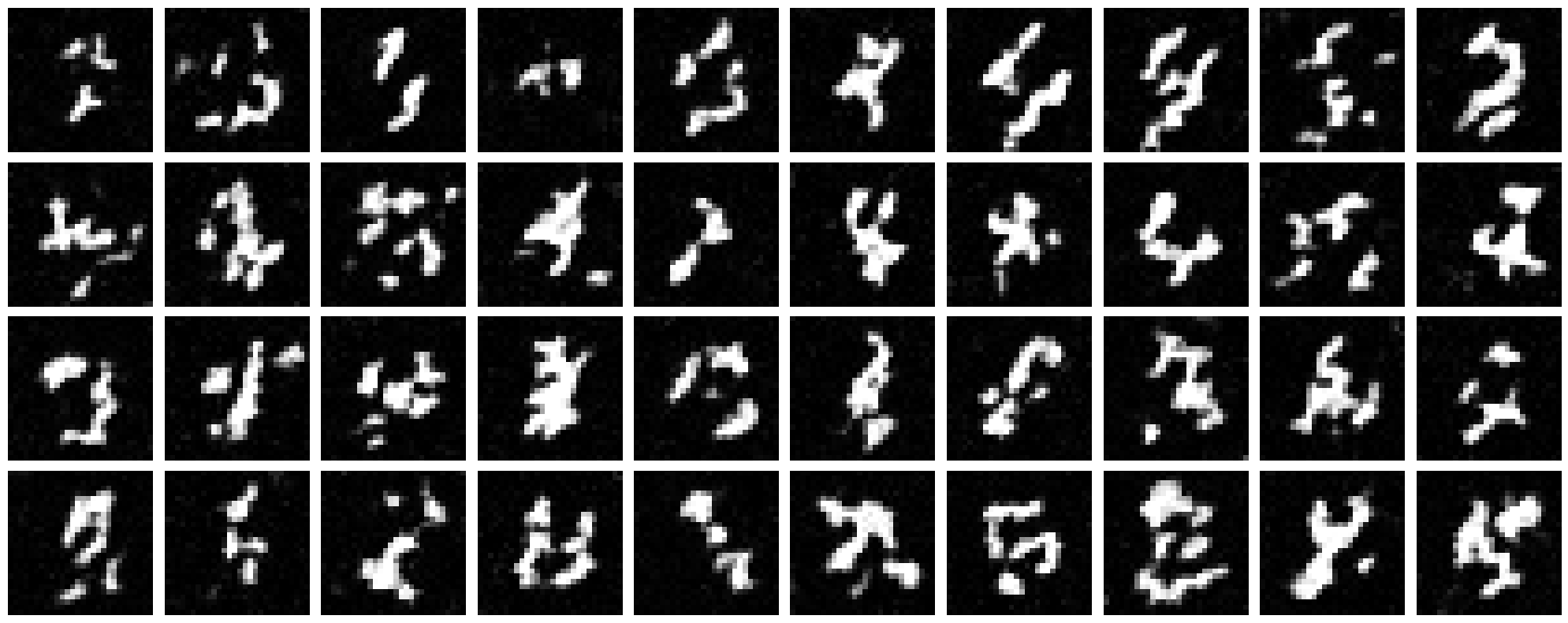
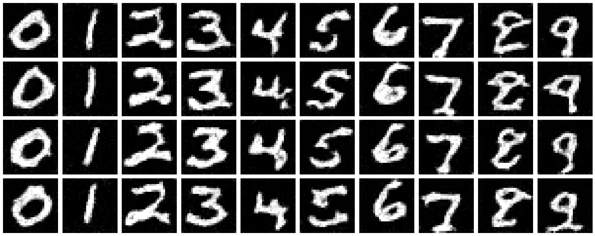
2.3 Sampling from the Time-Conditioned UNet
Using the trained time-conditioned UNet, I generated samples by starting from pure noise and iteratively applying the predicted flow. The results show significant improvement over single-step denoising, with recognizable digits emerging by epoch 10.
2.4 Class-Conditioned UNet
To improve generation quality and enable controlled generation, I extended the UNet to also condition on digit class (0-9). The class information is encoded as a one-hot vector and injected into the network through additional FCBlocks for class conditioning. This also requires implementing classifier-free guidance during both training and sampling.
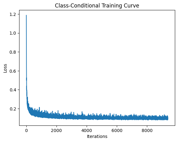
2.5 Training the Class-Conditioned UNet
I trained the class-conditioned model with different optimization strategies to compare their effectiveness. During training, 10% of samples use unconditional generation (class dropout) to enable classifier-free guidance.
Training with Learning Rate Scheduler
I trained the class-conditioned model with an exponential learning rate scheduler for improved convergence.
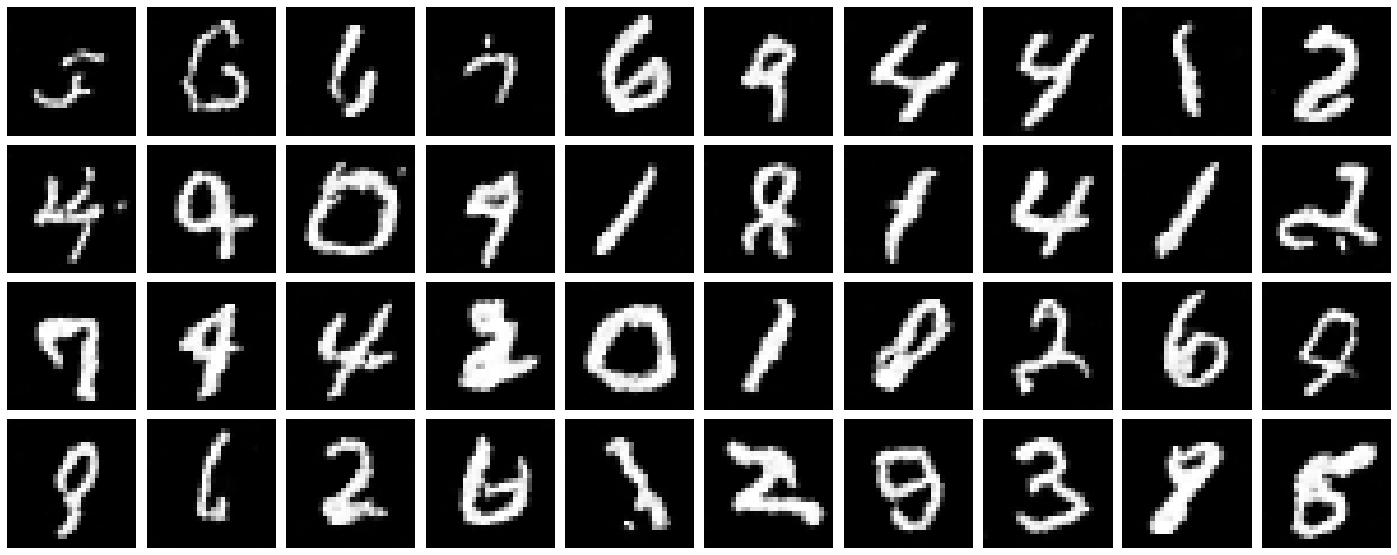
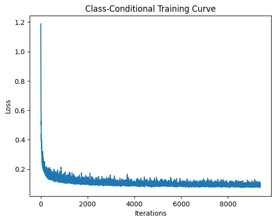
Training Without Learning Rate Scheduler
I also experimented with removing the exponential learning rate scheduler to see if similar performance could be achieved through architectural or optimization improvements. I maintained the same performance by adjusting the initial learning rate and using a learning rate of $lr = 0.0001$.
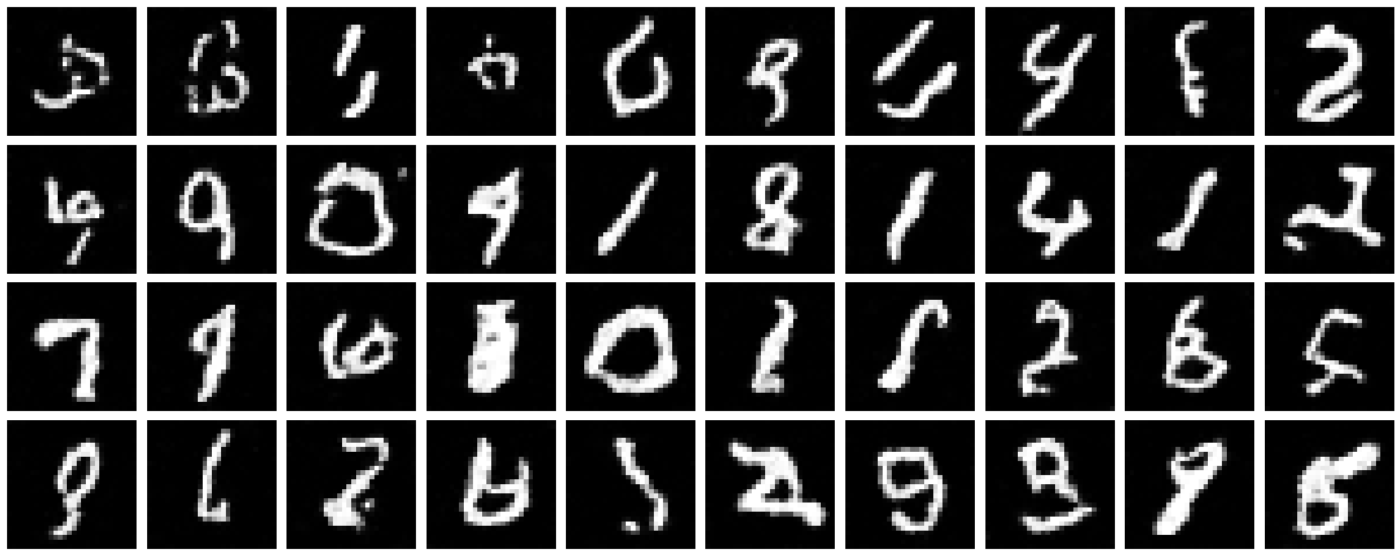
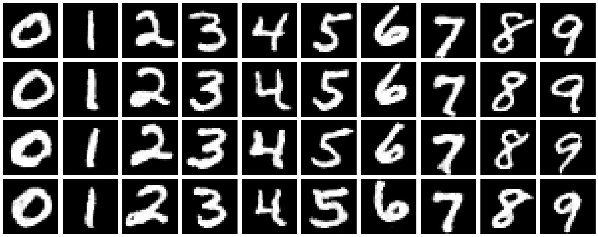
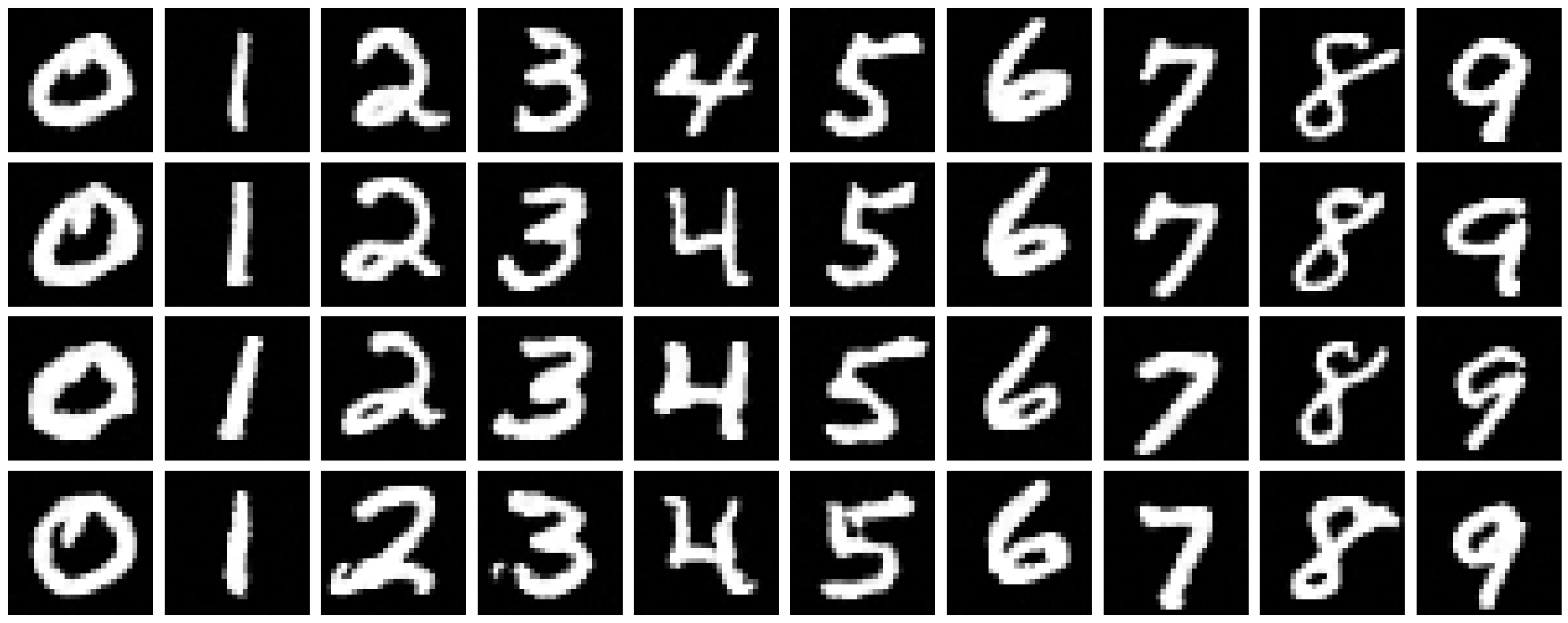
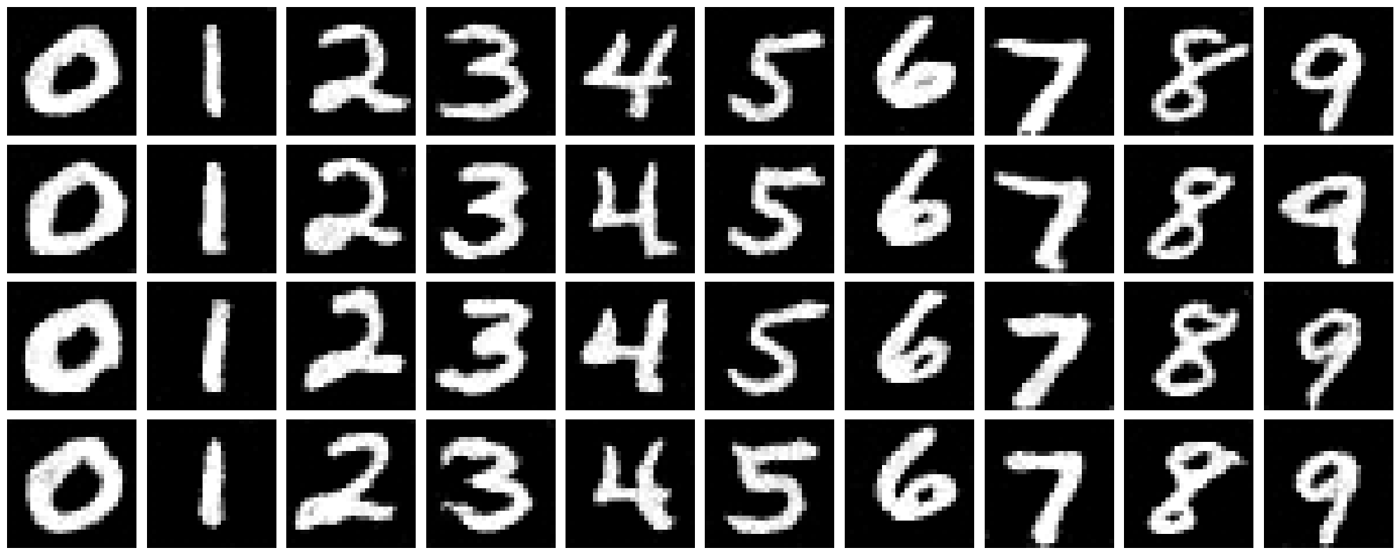
2.6 Sampling from the Class-Conditioned UNet
Using classifier-free guidance with $\gamma = 0.01$, I generated 4 instances of each digit (0-9). The class conditioning allows for much more controlled and higher-quality generation compared to the time-only model.
Results with Learning Rate Scheduler
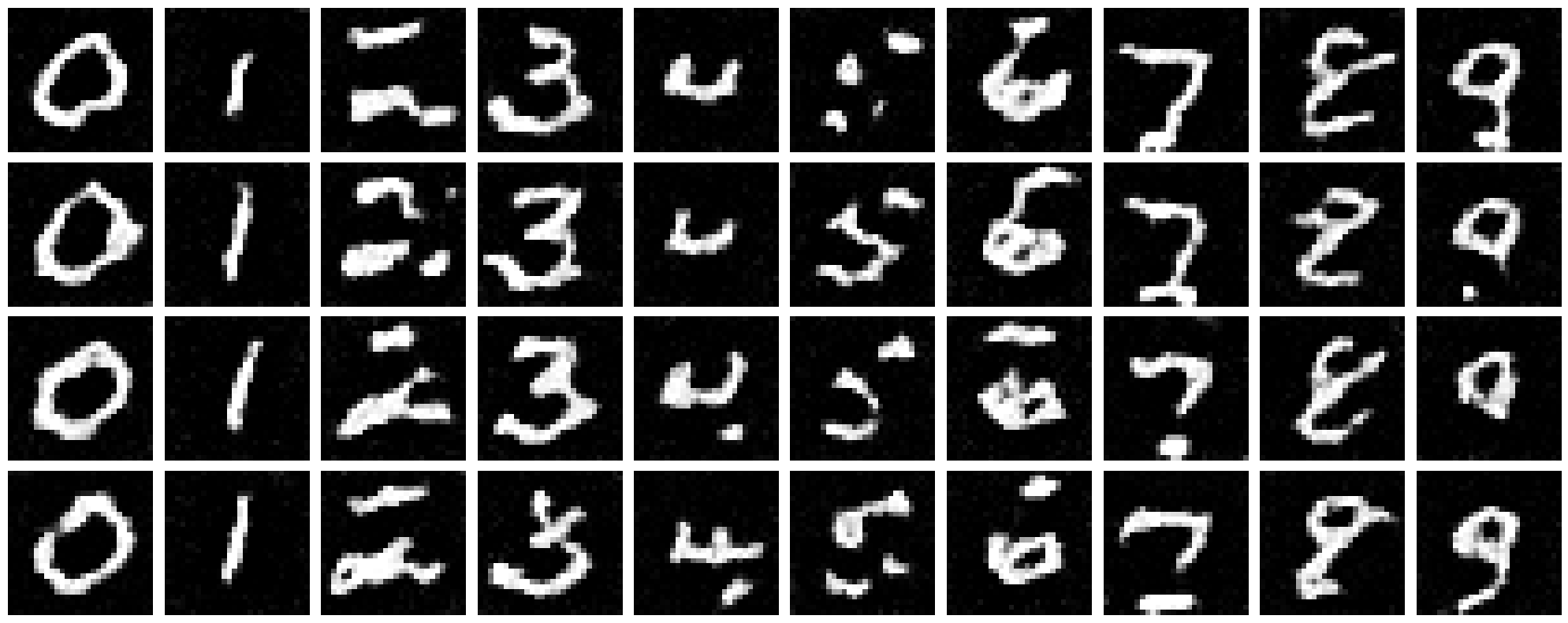
Results without Learning Rate Scheduler
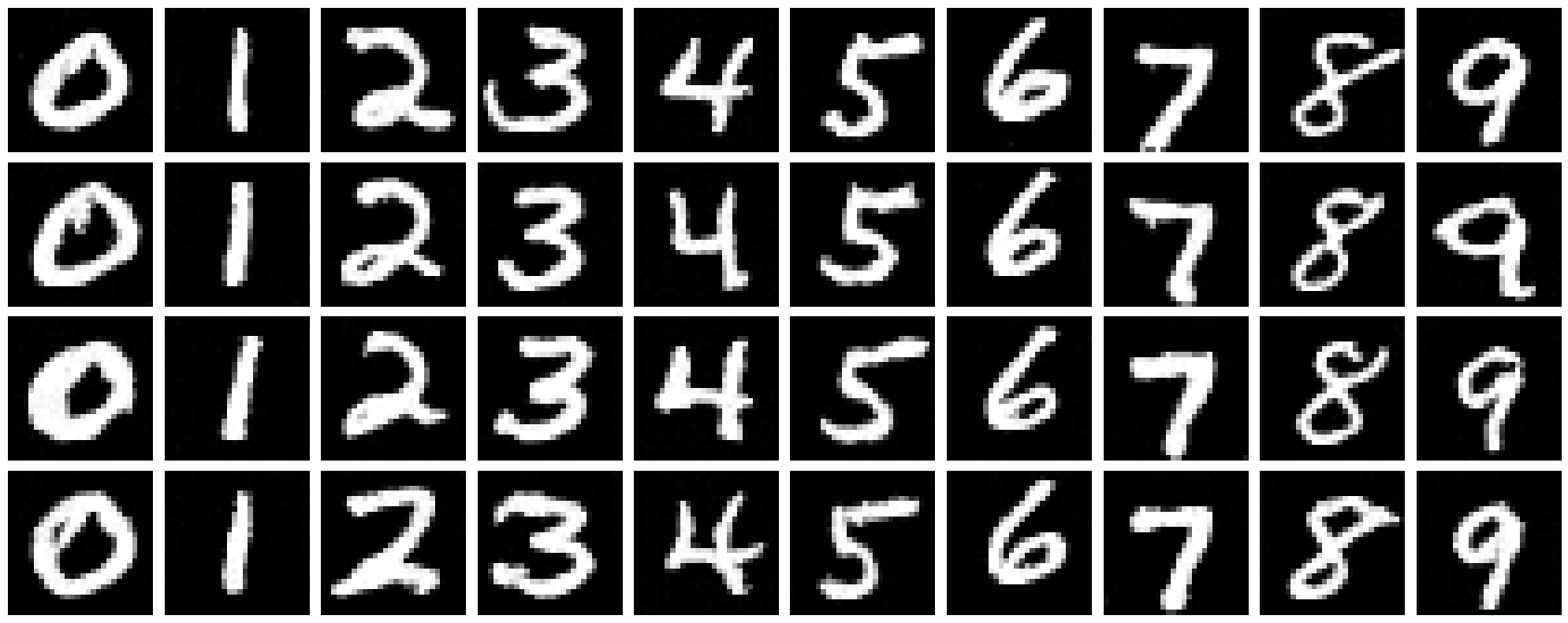
Even without the learning rate scheduler, by adjusting the initial learning rate to $lr = 0.0001$, the model achieved recognizable digit generation by epoch 10. Both approaches demonstrate the effectiveness of class conditioning for controlled generation.